Identification and classification of duplicated genes

Introduction

Gene and genome duplications are a source of raw genetic material for evolution (Ohno 2013). However, whole-genome duplications (WGD) and small-scale duplications (SSD) contribute to genome evolution in different manners. To help you explore the different contributions of WGD and SSD to evolution, we developed doubletrouble, a package that can be used to identify and classify duplicated genes from whole-genome protein sequences, calculate substitution rates per substitution site (i.e., $K_a$ and $K_s$ ) for gene pairs, find peaks in $K_s$ distributions, and classify gene pairs by age groups.

Installation

You can install doubletrouble from Bioconductor with the following code:

if(!requireNamespace("BiocManager", quietly = TRUE)) {
    install.packages("BiocManager")
}

BiocManager::install("doubletrouble")

## Check that you have a valid Bioconductor installation
BiocManager::valid()

Then, you can load the package:

library(doubletrouble)

Input data

To identify and classify duplicated gene pairs, users need two types of input data:

Whole-genome protein sequences (a.k.a. “proteome”), with only one protein sequence per gene (i.e., translated sequence of the primary transcript). These are typically stored in .fasta files.
Gene annotation, with genomic coordinates of all features (i.e., genes, exons, etc). These are typically stored in .gff3/.gff/.gtf files.
(Optional) Coding sequences (CDS), with only one DNA sequence sequence per gene. These are only required for users who want to calculate substitution rates (i.e., $K_a$ , $K_s$ , and their ratio $K_a/K_s$ ), and they are typically stored in .fasta files.

In the Bioconductor ecosystem, sequences and ranges are stored in standardized S4 classes named XStringSet (AAStringSet for proteins, DNAStringSet for DNA) and GRanges, respectively. This ensures seamless interoperability across packages, which is important for both users and package developers. Thus, doubletrouble expects proteomes in lists of AAStringSet objects, and annotations in lists of GRanges objects. Below you can find a summary of input data types, their typical file formats, and Bioconductor class.

Input data	File format	Bioconductor class	Requirement
Proteome	FASTA	`AAStringSet`	Mandatory
Annotation	GFF3/GTF	`GRanges`	Mandatory
CDS	FASTA	`DNAStringSet`	Optional

Names of list elements represent species identifiers (e.g., name, abbreviations, taxonomy IDs, or anything you like), and must be consistent across different lists, so correspondence can be made. For instance, suppose you have an object named seqs with a list of AAStringSet objects (proteomes for each species) named Athaliana, Alyrata, and Bnapus. You also have an object named annotation with a list of GRanges objects (gene annotation for each species). In this example, list names in annotation must also be Athaliana, Alyrata, and Bnapus (not necessarily in that order), so that doubletrouble knows that element Athaliana in seqs corresponds to element Athaliana in annotation. You can check that with:

# Checking if names of lists match
setequal(names(seqs), names(annotation)) # should return TRUE

IMPORTANT: If you have protein sequences as FASTA files in a directory, you can read them into a list of AAStringSet objects with the function fasta2AAStringSetlist() from the Bioconductor package syntenet. Likewise, you can get a GRangesList object from GFF/GTF files with the function gff2GRangesList(), also from syntenet.

Getting to know the example data sets

In this vignette, we will use data (proteome, gene annotations, and CDS) from the yeast species Saccharomyces cerevisiae and Candida glabrata, since their genomes are relatively small (and, hence, great for demonstration purposes). Our goal here is to identify and classify duplicated genes in the S. cerevisiae genome. The C. glabrata genome will be used as an outgroup to identify transposed duplicates later in this vignette.

Data were obtained from Ensembl Fungi release 54 (Yates et al. 2022). While you can download these data manually from the Ensembl Fungi webpage (or through another repository such as NCBI RefSeq), here we will demonstrate how you can get data from Ensembl using the biomartr package.

species <- c("Saccharomyces cerevisiae", "Candida glabrata")

# Download data from Ensembl with {biomartr}
## Whole-genome protein sequences (.fa)
fasta_dir <- file.path(tempdir(), "proteomes")
fasta_files <- biomartr::getProteomeSet(
    db = "ensembl", organisms = species, path = fasta_dir
)

## Gene annotation (.gff3)
gff_dir <- file.path(tempdir(), "annotation")
gff_files <- biomartr::getGFFSet(
    db = "ensembl", organisms = species, path = gff_dir
)

## CDS (.fa)
cds_dir <- file.path(tempdir(), "CDS")
cds_files <- biomartr::getCDSSet(
    db = "ensembl", organisms = species, path = cds_dir
)

# Import data to the R session
## Read .fa files with proteomes as a list of AAStringSet + clean names
seq <- syntenet::fasta2AAStringSetlist(fasta_dir)
names(seq) <- gsub("\\..*", "", names(seq))

## Read .gff3 files as a list of GRanges
annot <- syntenet::gff2GRangesList(gff_dir)
names(annot) <- gsub("\\..*", "", names(annot))

## Read .fa files with CDS as a list of DNAStringSet objects
cds <- lapply(cds_files, Biostrings::readDNAStringSet)
names(cds) <- gsub("\\..*", "", basename(cds_files))

# Process data
## Keep ranges for protein-coding genes only
yeast_annot <- lapply(annot, function(x) {
    gene_ranges <- x[x$biotype == "protein_coding" & x$type == "gene"]
    gene_ranges <- IRanges::subsetByOverlaps(x, gene_ranges)
    return(gene_ranges)
})

## Keep only longest sequence for each protein-coding gene (no isoforms)
yeast_seq <- lapply(seq, function(x) {
    # Keep only protein-coding genes
    x <- x[grep("protein_coding", names(x))]
    
    # Leave only gene IDs in sequence names
    names(x) <- gsub(".*gene:| .*", "", names(x))
    
    # If isoforms are present (same gene ID multiple times), keep the longest
    x <- x[order(Biostrings::width(x), decreasing = TRUE)]
    x <- x[!duplicated(names(x))]
    
    return(x)
})

Note that processing might differ depending on the data source. For instance, Ensembl adds gene ‘biotypes’ (e.g., protein-coding, pseudogene, etc) in sequence names and in a field named biotype in annotation files. Other databases might add these information elsewhere.

To avoid problems building this vignette (due to no/slow/unstable internet connection), the code chunk above is not executed. Instead, we ran such code and saved data in the following objects:

yeast_seq: A list of AAStringSet objects with elements named Scerevisiae and Cglabrata.
yeast_annot: A GRangesList object with elements named Scerevisiae and Cglabrata.

Let’s take a look at them.

# Load example data
data(yeast_seq)
data(yeast_annot)

yeast_seq
#> $Scerevisiae
#> AAStringSet object of length 6600:
#>        width seq                                            names               
#>    [1]  4910 MSQDRILLDLDVVNQRLILFNS...SELPEMLSLILRQYFTDLASS YLR106C
#>    [2]  4092 MCKNEARLANELIEFVAATVTG...NYERLQAKEVASSTEQLLQEM YKR054C
#>    [3]  3744 MSLTEQIEQFASRFRDDDATLQ...IGSAVSPRNLARTDVNFMPWF YHR099W
#>    [4]  3268 MVLFTRCEKARKEKLAAGYKPL...ETLRGSLLLAINEGHEGFGLA YDR457W
#>    [5]  3144 MLESLAANLLNRLLGSYVENFD...SLYRNIAIAVREYNKYCEAIL YLL040C
#>    ...   ... ...
#> [6596]    25 MFSLSNSQYTCQDYISDHIWKTSSH                      YOR302W
#> [6597]    25 MRAKWRKKRTRRLKRKRRKVRARSK                      YDL133C-A
#> [6598]    24 MHSNNSRQILIPHQNENMFLTELY                       YDL247W-A
#> [6599]    24 MLVLYRKRFSGFRFYFLSIFKYII                       YBR191W-A
#> [6600]    16 MLSLIFYLRFPSYIRG                               YJR151W-A
#> 
#> $Cglabrata
#> AAStringSet object of length 5293:
#>        width seq                                            names               
#>    [1]  4880 MSIQSADTVVFDLDKAFQRRDE...VELPEMLALILRQYFSDLASQ CAGL0M11616g
#>    [2]  4336 MYCIIRLCLLLLYMVRFAAAIV...ITFLGIKKCIILLIIVVVSIA CAGL0I10147g
#>    [3]  4041 MVQRNIELARYITTLLIGVCPK...NDIESKVLDDTKQLLNSIEYV CAGL0K08294g
#>    [4]  3743 MASADQISEYAEKLKDDQQSLA...ISASVNPRNLAKTDISFMPWF CAGL0A01914g
#>    [5]  3247 MVKLTRFEKLQKEKNAEYFKPF...DTLRGSLLIAINEGHEGFGLA CAGL0K06303g
#>    ...   ... ...
#> [5289]    43 MLGAPISRDTPRKTRSKTQFFQGPIVSLITEKCTYEWGNPSIN    CAGL0M02541g
#> [5290]    39 MLPGGPIVVLILVGLAACIIVATIIYRKWQERQRALARF        CAGL0M03305g
#> [5291]    39 MLPGGVILVFILVGLAACAIVAVIIYRKWQERQRSLQRF        CAGL0L08008g
#> [5292]    37 MINEGQLQTLVIGFGLAMVVLVVVYHAVASTMAVKRD          CAGL0C05461g
#> [5293]    34 MQPTIEATQKDNTQEKRDNYIVKGFFWSPDCVIA             CAGL0C01919g
yeast_annot
#> GRangesList object of length 2:
#> $Scerevisiae
#> GRanges object with 27144 ranges and 9 metadata columns:
#>           seqnames        ranges strand |       type     phase
#>              <Rle>     <IRanges>  <Rle> |   <factor> <integer>
#>       [1]        I      1-230218      * | chromosome      <NA>
#>       [2]        I       335-649      + | gene            <NA>
#>       [3]        I       335-649      + | mRNA            <NA>
#>       [4]        I       335-649      + | exon            <NA>
#>       [5]        I       335-649      + | CDS                0
#>       ...      ...           ...    ... .        ...       ...
#>   [27140]      XVI 944603-947701      + |       CDS          0
#>   [27141]      XVI 946856-947338      - |       gene      <NA>
#>   [27142]      XVI 946856-947338      - |       mRNA      <NA>
#>   [27143]      XVI 946856-947338      - |       exon      <NA>
#>   [27144]      XVI 946856-947338      - |       CDS          0
#>                               ID                 Parent              Name
#>                      <character>        <CharacterList>       <character>
#>       [1]           chromosome:I                                     <NA>
#>       [2]           gene:YAL069W                                     <NA>
#>       [3] transcript:YAL069W_m..           gene:YAL069W              <NA>
#>       [4]                   <NA> transcript:YAL069W_m..   YAL069W_mRNA-E1
#>       [5]            CDS:YAL069W transcript:YAL069W_m..              <NA>
#>       ...                    ...                    ...               ...
#>   [27140]            CDS:YPR204W transcript:YPR204W_m..              <NA>
#>   [27141]         gene:YPR204C-A                                     <NA>
#>   [27142] transcript:YPR204C-A..         gene:YPR204C-A              <NA>
#>   [27143]                   <NA> transcript:YPR204C-A.. YPR204C-A_mRNA-E1
#>   [27144]          CDS:YPR204C-A transcript:YPR204C-A..              <NA>
#>               gene_id  transcript_id           exon_id  protein_id
#>           <character>    <character>       <character> <character>
#>       [1]        <NA>           <NA>              <NA>        <NA>
#>       [2]     YAL069W           <NA>              <NA>        <NA>
#>       [3]        <NA>   YAL069W_mRNA              <NA>        <NA>
#>       [4]        <NA>           <NA>   YAL069W_mRNA-E1        <NA>
#>       [5]        <NA>           <NA>              <NA>     YAL069W
#>       ...         ...            ...               ...         ...
#>   [27140]        <NA>           <NA>              <NA>     YPR204W
#>   [27141]   YPR204C-A           <NA>              <NA>        <NA>
#>   [27142]        <NA> YPR204C-A_mRNA              <NA>        <NA>
#>   [27143]        <NA>           <NA> YPR204C-A_mRNA-E1        <NA>
#>   [27144]        <NA>           <NA>              <NA>   YPR204C-A
#>   -------
#>   seqinfo: 31 sequences from an unspecified genome; no seqlengths
#> 
#> $Cglabrata
#> GRanges object with 31671 ranges and 9 metadata columns:
#>                         seqnames      ranges strand |     type     phase
#>                            <Rle>   <IRanges>  <Rle> | <factor> <integer>
#>       [1] ChrA_C_glabrata_CBS138    1-491328      * |   region      <NA>
#>       [2] ChrA_C_glabrata_CBS138   1608-2636      - |   gene        <NA>
#>       [3] ChrA_C_glabrata_CBS138   1608-2636      - |   mRNA        <NA>
#>       [4] ChrA_C_glabrata_CBS138   1608-2636      - |   exon        <NA>
#>       [5] ChrA_C_glabrata_CBS138   1608-2636      - |   CDS            0
#>       ...                    ...         ...    ... .      ...       ...
#>   [31667] mito_C_glabrata_CBS138 15384-16067      + |     CDS          0
#>   [31668] mito_C_glabrata_CBS138 16756-17565      + |     gene      <NA>
#>   [31669] mito_C_glabrata_CBS138 16756-17565      + |     mRNA      <NA>
#>   [31670] mito_C_glabrata_CBS138 16756-17565      + |     exon      <NA>
#>   [31671] mito_C_glabrata_CBS138 16756-17565      + |     CDS          0
#>                               ID                 Parent              Name
#>                      <character>        <CharacterList>       <character>
#>       [1] region:ChrA_C_glabra..                                     <NA>
#>       [2]      gene:CAGL0A00105g                                     <NA>
#>       [3] transcript:CAGL0A001..      gene:CAGL0A00105g              <NA>
#>       [4]                   <NA> transcript:CAGL0A001.. CAGL0A00105g-T-E1
#>       [5]  CDS:CAGL0A00105g-T-p1 transcript:CAGL0A001..              <NA>
#>       ...                    ...                    ...               ...
#>   [31667]     CDS:CaglfMp11-T-p1 transcript:CaglfMp11-T              <NA>
#>   [31668]         gene:CaglfMp12                                     COX3
#>   [31669] transcript:CaglfMp12-T         gene:CaglfMp12              <NA>
#>   [31670]                   <NA> transcript:CaglfMp12-T    CaglfMp12-T-E1
#>   [31671]     CDS:CaglfMp12-T-p1 transcript:CaglfMp12-T              <NA>
#>                gene_id  transcript_id           exon_id        protein_id
#>            <character>    <character>       <character>       <character>
#>       [1]         <NA>           <NA>              <NA>              <NA>
#>       [2] CAGL0A00105g           <NA>              <NA>              <NA>
#>       [3]         <NA> CAGL0A00105g-T              <NA>              <NA>
#>       [4]         <NA>           <NA> CAGL0A00105g-T-E1              <NA>
#>       [5]         <NA>           <NA>              <NA> CAGL0A00105g-T-p1
#>       ...          ...            ...               ...               ...
#>   [31667]         <NA>           <NA>              <NA>    CaglfMp11-T-p1
#>   [31668]    CaglfMp12           <NA>              <NA>              <NA>
#>   [31669]         <NA>    CaglfMp12-T              <NA>              <NA>
#>   [31670]         <NA>           <NA>    CaglfMp12-T-E1              <NA>
#>   [31671]         <NA>           <NA>              <NA>    CaglfMp12-T-p1
#>   -------
#>   seqinfo: 31 sequences from an unspecified genome; no seqlengths

Data preparation

First of all, we need to process the list of protein sequences and gene ranges to detect synteny with syntenet. We will do that using the function process_input() from the syntenet package.

library(syntenet)

# Process input data
pdata <- process_input(yeast_seq, yeast_annot)

# Inspect the output
names(pdata)
#> [1] "seq"        "annotation"
pdata$seq
#> $Scerevisiae
#> AAStringSet object of length 6600:
#>        width seq                                            names               
#>    [1]  4910 MSQDRILLDLDVVNQRLILFNS...SELPEMLSLILRQYFTDLASS Sce_YLR106C
#>    [2]  4092 MCKNEARLANELIEFVAATVTG...NYERLQAKEVASSTEQLLQEM Sce_YKR054C
#>    [3]  3744 MSLTEQIEQFASRFRDDDATLQ...IGSAVSPRNLARTDVNFMPWF Sce_YHR099W
#>    [4]  3268 MVLFTRCEKARKEKLAAGYKPL...ETLRGSLLLAINEGHEGFGLA Sce_YDR457W
#>    [5]  3144 MLESLAANLLNRLLGSYVENFD...SLYRNIAIAVREYNKYCEAIL Sce_YLL040C
#>    ...   ... ...
#> [6596]    25 MFSLSNSQYTCQDYISDHIWKTSSH                      Sce_YOR302W
#> [6597]    25 MRAKWRKKRTRRLKRKRRKVRARSK                      Sce_YDL133C-A
#> [6598]    24 MHSNNSRQILIPHQNENMFLTELY                       Sce_YDL247W-A
#> [6599]    24 MLVLYRKRFSGFRFYFLSIFKYII                       Sce_YBR191W-A
#> [6600]    16 MLSLIFYLRFPSYIRG                               Sce_YJR151W-A
#> 
#> $Cglabrata
#> AAStringSet object of length 5293:
#>        width seq                                            names               
#>    [1]  4880 MSIQSADTVVFDLDKAFQRRDE...VELPEMLALILRQYFSDLASQ Cgl_CAGL0M11616g
#>    [2]  4336 MYCIIRLCLLLLYMVRFAAAIV...ITFLGIKKCIILLIIVVVSIA Cgl_CAGL0I10147g
#>    [3]  4041 MVQRNIELARYITTLLIGVCPK...NDIESKVLDDTKQLLNSIEYV Cgl_CAGL0K08294g
#>    [4]  3743 MASADQISEYAEKLKDDQQSLA...ISASVNPRNLAKTDISFMPWF Cgl_CAGL0A01914g
#>    [5]  3247 MVKLTRFEKLQKEKNAEYFKPF...DTLRGSLLIAINEGHEGFGLA Cgl_CAGL0K06303g
#>    ...   ... ...
#> [5289]    43 MLGAPISRDTPRKTRSKTQFFQGPIVSLITEKCTYEWGNPSIN    Cgl_CAGL0M02541g
#> [5290]    39 MLPGGPIVVLILVGLAACIIVATIIYRKWQERQRALARF        Cgl_CAGL0M03305g
#> [5291]    39 MLPGGVILVFILVGLAACAIVAVIIYRKWQERQRSLQRF        Cgl_CAGL0L08008g
#> [5292]    37 MINEGQLQTLVIGFGLAMVVLVVVYHAVASTMAVKRD          Cgl_CAGL0C05461g
#> [5293]    34 MQPTIEATQKDNTQEKRDNYIVKGFFWSPDCVIA             Cgl_CAGL0C01919g
pdata$annotation
#> $Scerevisiae
#> GRanges object with 6600 ranges and 1 metadata column:
#>          seqnames        ranges strand |          gene
#>             <Rle>     <IRanges>  <Rle> |   <character>
#>      [1]    Sce_I       335-649      + |   Sce_YAL069W
#>      [2]    Sce_I       538-792      + | Sce_YAL068W-A
#>      [3]    Sce_I     1807-2169      - |   Sce_YAL068C
#>      [4]    Sce_I     2480-2707      + | Sce_YAL067W-A
#>      [5]    Sce_I     7235-9016      - |   Sce_YAL067C
#>      ...      ...           ...    ... .           ...
#>   [6596]  Sce_XVI 939922-941136      + |   Sce_YPR201W
#>   [6597]  Sce_XVI 943032-943896      + |   Sce_YPR202W
#>   [6598]  Sce_XVI 943880-944188      + |   Sce_YPR203W
#>   [6599]  Sce_XVI 944603-947701      + |   Sce_YPR204W
#>   [6600]  Sce_XVI 946856-947338      - | Sce_YPR204C-A
#>   -------
#>   seqinfo: 17 sequences from an unspecified genome; no seqlengths
#> 
#> $Cglabrata
#> GRanges object with 5293 ranges and 1 metadata column:
#>                        seqnames      ranges strand |             gene
#>                           <Rle>   <IRanges>  <Rle> |      <character>
#>      [1] Cgl_ChrA_C_glabrata_..   1608-2636      - | Cgl_CAGL0A00105g
#>      [2] Cgl_ChrA_C_glabrata_..   2671-4809      - | Cgl_CAGL0A00116g
#>      [3] Cgl_ChrA_C_glabrata_.. 11697-13042      + | Cgl_CAGL0A00132g
#>      [4] Cgl_ChrA_C_glabrata_.. 14977-15886      + | Cgl_CAGL0A00154g
#>      [5] Cgl_ChrA_C_glabrata_.. 17913-19017      - | Cgl_CAGL0A00165g
#>      ...                    ...         ...    ... .              ...
#>   [5289] Cgl_mito_C_glabrata_.. 13275-13421      + |    Cgl_CaglfMp08
#>   [5290] Cgl_mito_C_glabrata_.. 13614-14396      + |    Cgl_CaglfMp09
#>   [5291] Cgl_mito_C_glabrata_.. 14631-14861      + |    Cgl_CaglfMp10
#>   [5292] Cgl_mito_C_glabrata_.. 15384-16067      + |    Cgl_CaglfMp11
#>   [5293] Cgl_mito_C_glabrata_.. 16756-17565      + |    Cgl_CaglfMp12
#>   -------
#>   seqinfo: 14 sequences from an unspecified genome; no seqlengths

The processed data are represented as a list with the elements seq and annotation, each containing the protein sequences and gene ranges for each species, respectively.

Finally, we need to perform pairwise sequence similarity searches to identify the whole set of paralogous gene pairs. We can do this using the function run_diamond() from the syntenet package ¹, setting compare = "intraspecies" to perform only intraspecies comparisons.

data(diamond_intra)

# Run DIAMOND in sensitive mode for S. cerevisiae only
if(diamond_is_installed()) {
    diamond_intra <- run_diamond(
        seq = pdata$seq["Scerevisiae"],
        compare = "intraspecies", 
        outdir = file.path(tempdir(), "diamond_intra"),
        ... = "--sensitive"
    )
}

# Inspect output
names(diamond_intra)
#> [1] "Scerevisiae_Scerevisiae"
head(diamond_intra$Scerevisiae_Scerevisiae)
#>         query          db perc_identity length mismatches gap_open qstart qend
#> 1 Sce_YLR106C Sce_YLR106C         100.0   4910          0        0      1 4910
#> 2 Sce_YLR106C Sce_YKR054C          22.4    420        254       19    804 1195
#> 3 Sce_YKR054C Sce_YKR054C         100.0   4092          0        0      1 4092
#> 4 Sce_YKR054C Sce_YLR106C          22.4    420        254       19   1823 2198
#> 5 Sce_YHR099W Sce_YHR099W         100.0   3744          0        0      1 3744
#> 6 Sce_YHR099W Sce_YJR066W          22.7    339        201       12   3351 3674
#>   tstart tend   evalue bitscore
#> 1      1 4910 0.00e+00   9095.0
#> 2   1823 2198 1.30e-06     53.1
#> 3      1 4092 0.00e+00   7940.0
#> 4    804 1195 1.09e-06     53.1
#> 5      1 3744 0.00e+00   7334.0
#> 6   2074 2366 6.46e-08     57.0

And voilà! Now that we have the DIAMOND output and the processed annotation, you can classify the duplicated genes.

Classifying duplicated gene pairs and genes

To classify duplicated gene pairs based on their modes of duplication, you will use the function classify_gene_pairs(). This function offers four different classification schemes, depending on how much detail you want. The classification schemes, along with the duplication modes they identify and their required input, are summarized in the table below:

Scheme	Duplication modes	Required input
binary	SD, SSD	`blast_list`, `annotation`
standard	SD, TD, PD, DD	`blast_list`, `annotation`
extended	SD, TD, PD, TRD, DD	`blast_list`, `annotation`, `blast_inter`
full	SD, TD, PD, rTRD, dTRD, DD	`blast_list`, `annotation`, `blast_inter`, `intron_counts`

Legend: SD, segmental duplication. SSD, small-scale duplication. TD, tandem duplication. PD, proximal duplication. TRD, transposon-derived duplication. rTRD, retrotransposon-derived duplication. dTRD, DNA transposon-derived duplication. DD, dispersed duplication.

As shown in the table, the minimal input objects are:

blast_list: A list of data frames with DIAMOND (or BLASTp, etc.) tabular output for intraspecies comparisons as returned by syntenet::run_diamond(..., compare = 'intraspecies').
annotation: The processed annotation list (a GRangesList object) as returned by syntenet::process_input().

However, if you also want to identify transposon-derived duplicates (TRD) and further classify them as retrotransposon-derived duplicates (rTRD) or DNA transposon-derived duplicates (dTRD), you will need the following objects:

blast_list: A list of data frames with DIAMOND (or BLASTp, etc.) tabular output for interspecies comparisons (target species vs an outgroup) as returned by syntenet::run_diamond(..., compare = <comparison_data_frame>).
intron_counts: A list of data frames with the number of introns per gene for each species, as returned by get_intron_counts().

Below, we demonstrate each classification scheme with examples.

The binary scheme (SD vs SSD)

The binary scheme classifies duplicates as derived from either segmental duplications (SD) or small-scale duplications (SSD). To identify segmental duplicates, the function classify_gene_pairs() performs intragenome synteny detection scans with syntenet and classifies any detected anchor pairs as segmental duplicates. The remaining pairs are classified as originating from small-scale duplications.

This scheme can be used by specifying scheme = "binary" in the function classify_gene_pairs().

# Binary scheme
c_binary <- classify_gene_pairs(
    annotation = pdata$annotation,
    blast_list = diamond_intra,
    scheme = "binary"
)

# Inspecting the output
names(c_binary)
#> [1] "Scerevisiae"
head(c_binary$Scerevisiae)
#>           dup1        dup2 type
#> 9  Sce_YDR457W Sce_YER125W  SSD
#> 10 Sce_YDR457W Sce_YJR036C  SSD
#> 11 Sce_YDR457W Sce_YGL141W  SSD
#> 12 Sce_YDR457W Sce_YKL010C  SSD
#> 15 Sce_YBR140C Sce_YOL081W  SSD
#> 21 Sce_YBL088C Sce_YBR136W  SSD

# How many pairs are there for each duplication mode?
table(c_binary$Scerevisiae$type)
#> 
#>   SD  SSD 
#>  342 3246

The function returns a list of data frames, each containing the duplicated gene pairs and their modes of duplication for each species (here, because we have only one species, this is a list of length 1).

The standard scheme (SSD → TD, PD, DD)

Gene pairs derived from small-scale duplications can be further classified as originating from tandem duplications (TD, genes are adjacent to each other), proximal duplications (PD, genes are separated by only a few genes), or dispersed duplications (DD, duplicates that do not fit in any of the previous categories).

This is the default classification scheme in classify_gene_pairs(), and it can be specified by setting scheme = "standard".

# Standard scheme
c_standard <- classify_gene_pairs(
    annotation = pdata$annotation,
    blast_list = diamond_intra,
    scheme = "standard"
)

# Inspecting the output
names(c_standard)
#> [1] "Scerevisiae"
head(c_standard$Scerevisiae)
#>            dup1        dup2 type
#> 124 Sce_YGR032W Sce_YLR342W   SD
#> 176 Sce_YOR396W Sce_YPL283C   SD
#> 189 Sce_YJL225C Sce_YIL177C   SD
#> 275 Sce_YNR031C Sce_YCR073C   SD
#> 285 Sce_YOR326W Sce_YAL029C   SD
#> 312 Sce_YJL222W Sce_YIL173W   SD

# How many pairs are there for each duplication mode?
table(c_standard$Scerevisiae$type)
#> 
#>   SD   TD   PD   DD 
#>  342   42   80 3124

The extended scheme (SSD → TD, PD, TRD, DD)

To find transposon-derived duplicates (TRD), the function classify_gene_pairs() detects syntenic regions between a target species and an outgroup species. Genes in the target species that are in syntenic regions with the outgroup are treated as ancestral loci. Then, if only one gene of the duplicate pair is an ancestral locus, this duplicate pair is classified as originating from transposon-derived duplications.

Since finding transposon-derived duplicates requires comparing a target species with an outgroup species, you will first need to perform a similarity search of your target species against an outgroup. You can do this with syntenet::run_diamond(). For the parameter compare, you will pass a 2-column data frame specifying the comparisons to be made. ²

Here, we will identify duplicated gene pairs for Saccharomyces cerevisiae using Candida glabrata as an outgroup.

data(diamond_inter) # load pre-computed output in case DIAMOND is not installed

# Create data frame of comparisons to be made
comparisons <- data.frame(
    species = "Scerevisiae",
    outgroup = "Cglabrata"
)
comparisons
#>       species  outgroup
#> 1 Scerevisiae Cglabrata

# Run DIAMOND for the comparison we specified
if(diamond_is_installed()) {
    diamond_inter <- run_diamond(
        seq = pdata$seq,
        compare = comparisons,
        outdir = file.path(tempdir(), "diamond_inter"),
        ... = "--sensitive"
    )
}

names(diamond_inter)
#> [1] "Scerevisiae_Cglabrata"
head(diamond_inter$Scerevisiae_Cglabrata)
#>         query               db perc_identity length mismatches gap_open qstart
#> 1 Sce_YLR106C Cgl_CAGL0M11616g          52.3   4989       2183       50      2
#> 2 Sce_YLR106C Cgl_CAGL0K08294g          23.1    347        215       12   1064
#> 3 Sce_YKR054C Cgl_CAGL0K08294g          26.5   4114       2753       81     83
#> 4 Sce_YKR054C Cgl_CAGL0M11616g          22.7    419        254       17   1823
#> 5 Sce_YHR099W Cgl_CAGL0A01914g          70.2   3761       1087       17      1
#> 6 Sce_YDR457W Cgl_CAGL0K06303g          55.5   3318       1355       39      1
#>   qend tstart tend   evalue bitscore
#> 1 4909      5 4879 0.00e+00   4439.0
#> 2 1389   1770 2085 9.10e-07     53.5
#> 3 4089     87 4035 0.00e+00   1376.0
#> 4 2198    803 1194 7.59e-07     53.5
#> 5 3744      1 3743 0.00e+00   5200.0
#> 6 3268      1 3247 0.00e+00   3302.0

Now, we will pass this interspecies DIAMOND output as an argument to the parameter blast_inter of classify_gene_pairs().

# Extended scheme
c_extended <- classify_gene_pairs(
    annotation = pdata$annotation,
    blast_list = diamond_intra,
    scheme = "extended",
    blast_inter = diamond_inter
)

# Inspecting the output
names(c_extended)
#> [1] "Scerevisiae"
head(c_extended$Scerevisiae)
#>            dup1        dup2 type
#> 124 Sce_YGR032W Sce_YLR342W   SD
#> 176 Sce_YOR396W Sce_YPL283C   SD
#> 189 Sce_YJL225C Sce_YIL177C   SD
#> 275 Sce_YNR031C Sce_YCR073C   SD
#> 285 Sce_YOR326W Sce_YAL029C   SD
#> 312 Sce_YJL222W Sce_YIL173W   SD

# How many pairs are there for each duplication mode?
table(c_extended$Scerevisiae$type)
#> 
#>   SD   TD   PD  TRD   DD 
#>  342   42   80 1015 2109

In the example above, we used only one outgroup species (C. glabrata). However, since results might change depending on the chosen outgroup, you can also use multiple outgroups in the comparisons data frame, and then run interspecies DIAMOND searches as above. For instance, suppose you want to use speciesB, speciesC, and speciesD as outgroups to speciesA. In this case, your data frame of comparisons (to be passed to the compare argument of syntenet::run_diamond()) would look like the following:

# Example: multiple outgroups for the same species
comparisons <- data.frame(
    species = rep("speciesA", 3),
    outgroup = c("speciesB", "speciesC", "speciesD")
)

comparisons
#>    species outgroup
#> 1 speciesA speciesB
#> 2 speciesA speciesC
#> 3 speciesA speciesD

When multiple outgroups are present, classify_gene_pairs() will check if gene pairs are classified as transposed (i.e., only one gene is an ancestral locus) in each of the outgroup species, and then calculate the percentage of outgroup species in which each pair is considered ‘transposed’. For instance, you could have gene pair 1 as transposed based on 30% of the outgroup species, gene pair 2 as transposed based on 100% of the outgroup species, gene pair 3 based on 0% of the outgroup species, and so on. By default, pairs are considered ‘transposed’ if they are classified as such in >70% of the outgroups, but you can choose a different minimum percentage cut-off using parameter outgroup_coverage.

The full scheme (SSD → TD, PD, rTRD, dTRD, DD)

Finally, the full scheme consists in classifying transposon-derived duplicates (TRD) further as originating from retrotransposons (rTRD) or DNA transposons (dTRD). To do that, the function classify_gene_pairs() uses the number of introns per gene to find TRD pairs for which one gene has at least 1 intron, and the other gene has no introns; if that is the case, the pair is classified as originating from the activity of retrotransposons (rTRD, i.e., the transposed gene without introns is a processed transcript that was retrotransposed back to the genome). All the other TRD pairs are classified as DNA transposon-derived duplicates (dTRD).

To classify duplicates using this scheme, you will first need to create a list of data frames with the number of introns per gene for each species. This can be done with the function get_intron_counts(), which takes a TxDb object as input. TxDb objects store transcript annotations, and they can be created with a family of functions named makeTxDbFrom* from the txdbmaker package (see ?get_intron_counts() for a summary of all functions).

Here, we will create a list of TxDb objects from a list of GRanges objects using the function makeTxDbFromGRanges() from txdbmaker. Importantly, to create a TxDb from a GRanges, the GRanges object must contain genomic coordinates for all features, including transcripts, exons, etc. Because of that, we will use annotation from the example data set yeast_annot, which was not processed with syntenet::process_input().

library(txdbmaker)
# Create a list of `TxDb` objects from a list of `GRanges` objects
txdb_list <- lapply(yeast_annot, txdbmaker::makeTxDbFromGRanges)
txdb_list
#> $Scerevisiae
#> TxDb object:
#> # Db type: TxDb
#> # Supporting package: GenomicFeatures
#> # Genome: NA
#> # Nb of transcripts: 6631
#> # Db created by: txdbmaker package from Bioconductor
#> # Creation time: 2024-10-07 14:08:27 +0000 (Mon, 07 Oct 2024)
#> # txdbmaker version at creation time: 1.1.1
#> # RSQLite version at creation time: 2.3.7
#> # DBSCHEMAVERSION: 1.2
#> 
#> $Cglabrata
#> TxDb object:
#> # Db type: TxDb
#> # Supporting package: GenomicFeatures
#> # Genome: NA
#> # Nb of transcripts: 5389
#> # Db created by: txdbmaker package from Bioconductor
#> # Creation time: 2024-10-07 14:08:27 +0000 (Mon, 07 Oct 2024)
#> # txdbmaker version at creation time: 1.1.1
#> # RSQLite version at creation time: 2.3.7
#> # DBSCHEMAVERSION: 1.2

Once we have the TxDb objects, we can get intron counts per gene with get_intron_counts().

# Get a list of data frames with intron counts per gene for each species
intron_counts <- lapply(txdb_list, get_intron_counts)

# Inspecting the list
names(intron_counts)
#> [1] "Scerevisiae" "Cglabrata"
head(intron_counts$Scerevisiae)
#>    gene introns
#> 1 Q0045       7
#> 2 Q0105       5
#> 3 Q0070       4
#> 4 Q0065       3
#> 5 Q0120       3
#> 6 Q0060       2

Finally, we can use this list to classify duplicates using the full scheme as follows:

# Full scheme
c_full <- classify_gene_pairs(
    annotation = pdata$annotation,
    blast_list = diamond_intra,
    scheme = "full",
    blast_inter = diamond_inter,
    intron_counts = intron_counts
)

# Inspecting the output
names(c_full)
#> [1] "Scerevisiae"
head(c_full$Scerevisiae)
#>            dup1        dup2 type
#> 124 Sce_YGR032W Sce_YLR342W   SD
#> 176 Sce_YOR396W Sce_YPL283C   SD
#> 189 Sce_YJL225C Sce_YIL177C   SD
#> 275 Sce_YNR031C Sce_YCR073C   SD
#> 285 Sce_YOR326W Sce_YAL029C   SD
#> 312 Sce_YJL222W Sce_YIL173W   SD

# How many pairs are there for each duplication mode?
table(c_full$Scerevisiae$type)
#> 
#>   SD   TD   PD rTRD dTRD   DD 
#>  342   42   80   52  963 2109

Classifying genes into unique modes of duplication

If you look carefully at the output of classify_gene_pairs(), you will notice that some genes appear in more than one duplicate pair, and these pairs can have different duplication modes assigned. There’s nothing wrong with it. Consider, for example, a gene that was originated by a segmental duplication some 60 million years ago, and then it underwent a tandem duplication 5 million years ago. In the output of classify_gene_pairs(), you’d see this gene in two pairs, one with SD in the type column, and one with TD.

If you want to assign each gene to a unique mode of duplication, you can use the function classify_genes(). This function assigns duplication modes hierarchically using factor levels in column type as the priority order. The priority orders for each classification scheme are:

Binary: SD > SSD.
Standard: SD > TD > PD > DD.
Extended: SD > TD > PD > TRD > DD.
Full: SD > TD > PD > rTRD > dTRD > DD.

The input for classify_genes() is the list of gene pairs returned by classify_gene_pairs().

# Classify genes into unique modes of duplication
c_genes <- classify_genes(c_full)

# Inspecting the output
names(c_genes)
#> [1] "Scerevisiae"
head(c_genes$Scerevisiae)
#>          gene type
#> 1 Sce_YGR032W   SD
#> 2 Sce_YOR396W   SD
#> 3 Sce_YJL225C   SD
#> 4 Sce_YNR031C   SD
#> 5 Sce_YOR326W   SD
#> 6 Sce_YJL222W   SD

# Number of genes per mode
table(c_genes$Scerevisiae$type)
#> 
#>   SD   TD   PD rTRD dTRD   DD 
#>  683   67   70   71  883  836

Calculating substitution rates for duplicated gene pairs

You can use the function pairs2kaks() to calculate rates of nonsynonymous substitutions per nonsynonymous site ( $K_a$ ), synonymouys substitutions per synonymous site ( $K_s$ ), and their ratios ( $K_a/K_s$ ). These rates are calculated using the Bioconductor package MSA2dist, which implements all codon models in KaKs_Calculator 2.0 (Wang et al. 2010).

For the purpose of demonstration, we will only calculate $K_a$ , $K_s$ , and $K_a/K_s$ for 5 TD-derived gene pairs. The CDS for TD-derived genes were obtained from Ensembl Fungi (Yates et al. 2022), and they are stored in cds_scerevisiae.

data(cds_scerevisiae)
head(cds_scerevisiae)
#> DNAStringSet object of length 6:
#>     width seq                                               names               
#> [1]  3486 ATGGTTAATATAAGCATCGTAGC...TTGTCGCTTTATTACTGCTATAG YJR151C
#> [2]  3276 ATGGGCGAAGGAACTACTAAGGA...TTAATATTGGTATTAAACAATGA YDR040C
#> [3]  3276 ATGAGCGAGGGAACTGTCAAAGA...TTAATATCAGTGTCAAGCATTAA YDR038C
#> [4]  3276 ATGAGCGAGGGAACTGTCAAAGA...TTAATATTGGTATTAAACAATGA YDR039C
#> [5]  2925 ATGAACAGTATGGCCGATACCGA...CCATTACAACATTTCAAACATAA YAR019C
#> [6]  2646 ATGCTGGAGTTTCCAATATCAGT...TAGCTGTTCTGTTCGCCTTCTAG YJL078C

# Store DNAStringSet object in a list
cds_list <- list(Scerevisiae = cds_scerevisiae)

# Keep only top five TD-derived gene pairs for demonstration purposes
td_pairs <- c_full$Scerevisiae[c_full$Scerevisiae$type == "TD", ]
gene_pairs <- list(Scerevisiae = td_pairs[seq(1, 5, by = 1), ])

# Calculate Ka, Ks, and Ka/Ks
kaks <- pairs2kaks(gene_pairs, cds_list)

# Inspect the output
head(kaks)
#> $Scerevisiae
#>    dup1  dup2       Ka       Ks    Ka_Ks type
#> 1 Q0055 Q0060      NaN      NaN      NaN   TD
#> 2 Q0065 Q0060 0.799925 3.549370 0.225371   TD
#> 3 Q0070 Q0045 0.296216 0.438575 0.675405   TD
#> 4 Q0070 Q0065 0.394617 0.582050 0.677977   TD
#> 5 Q0055 Q0050 0.629343 4.257430 0.147822   TD

Importantly, pairs2kaks() expects all genes in the gene pairs to be present in the CDS, with matching names. Species abbreviations in gene pairs (added by syntenet) are automatically removed, so you should not add them to the sequence names of your CDS.

Identifying and visualizing $K_s$ peaks

Peaks in $K_s$ distributions typically indicate whole-genome duplication (WGD) events, and they can be identified by fitting Gaussian mixture models (GMMs) to $K_s$ distributions. In doubletrouble, this can be performed with the function find_ks_peaks().

However, because of saturation at higher $K_s$ values, only recent WGD events can be reliably identified from $K_s$ distributions (Vanneste, Van de Peer, and Maere 2013). Recent WGD events are commonly found in plant species, such as maize, soybean, apple, etc. Although the genomes of yeast species have signatures of WGD, these events are ancient, so it is very hard to find evidence for them using $K_s$ distributions. ³

To demonstrate how you can find peaks in $K_s$ distributions with find_ks_peaks(), we will use a data frame containing $K_s$ values for duplicate pairs in the soybean (Glycine max) genome, which has undergone 2 WGDs events ~13 and ~58 million years ago (Schmutz et al. 2010). Then, we will visualize $K_s$ distributions with peaks using the function plot_ks_peaks().

First of all, let’s look at the data and have a quick look at the distribution with the function plot_ks_distro() (more details on this function in the data visualization section).

# Load data and inspect it
data(gmax_ks)
head(gmax_ks)
#>              dup1            dup2     Ks type
#> 1 GLYMA_07G035600 GLYMA_16G004800 0.1670   SD
#> 2 GLYMA_18G275200 GLYMA_08G252600 0.1070   SD
#> 3 GLYMA_09G282200 GLYMA_20G003400 0.0822   SD
#> 4 GLYMA_01G166400 GLYMA_11G077000 0.0904   SD
#> 5 GLYMA_07G252100 GLYMA_17G022300 0.1400   SD
#> 6 GLYMA_05G133100 GLYMA_08G087600 0.0883   SD

# Plot distribution
plot_ks_distro(gmax_ks)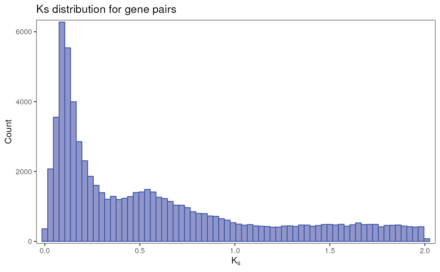

By visual inspection, we can see 2 or 3 peaks. Based on our prior knowledge, we know that 2 WGD events have occurred in the ancestral of the Glycine genus and in the ancestral of all Fabaceae, which seem to correspond to the peaks we see at $K_s$ values around 0.1 and 0.5, respectively. There could be a third, flattened peak at around 1.6, which would represent the WGD shared by all eudicots. Let’s test which number of peaks has more support: 2 or 3.

# Find 2 and 3 peaks and test which one has more support
peaks <- find_ks_peaks(gmax_ks$Ks, npeaks = c(2, 3), verbose = TRUE)
#> Optimal number of peaks: 3
#> Bayesian Information Criterion (BIC): 
#>            E         V
#> 2 -100166.88 -88545.37
#> 3  -90965.45 -75323.66
#> 
#> Top 3 models based on the BIC criterion: 
#>       V,3       V,2       E,3 
#> -75323.66 -88545.37 -90965.45
names(peaks)
#> [1] "mean"   "sd"     "lambda" "ks"
str(peaks)
#> List of 4
#>  $ mean  : Named num [1:3] 0.123 0.601 1.596
#>   ..- attr(*, "names")= chr [1:3] "1" "2" "3"
#>  $ sd    : num [1:3] 0.0572 0.287 0.2503
#>  $ lambda: num [1:3] 0.285 0.44 0.276
#>  $ ks    : num [1:68085] 0.167 0.107 0.0822 0.0904 0.14 0.0883 0.107 0.756 0.737 0.0872 ...

# Visualize Ks distribution
plot_ks_peaks(peaks)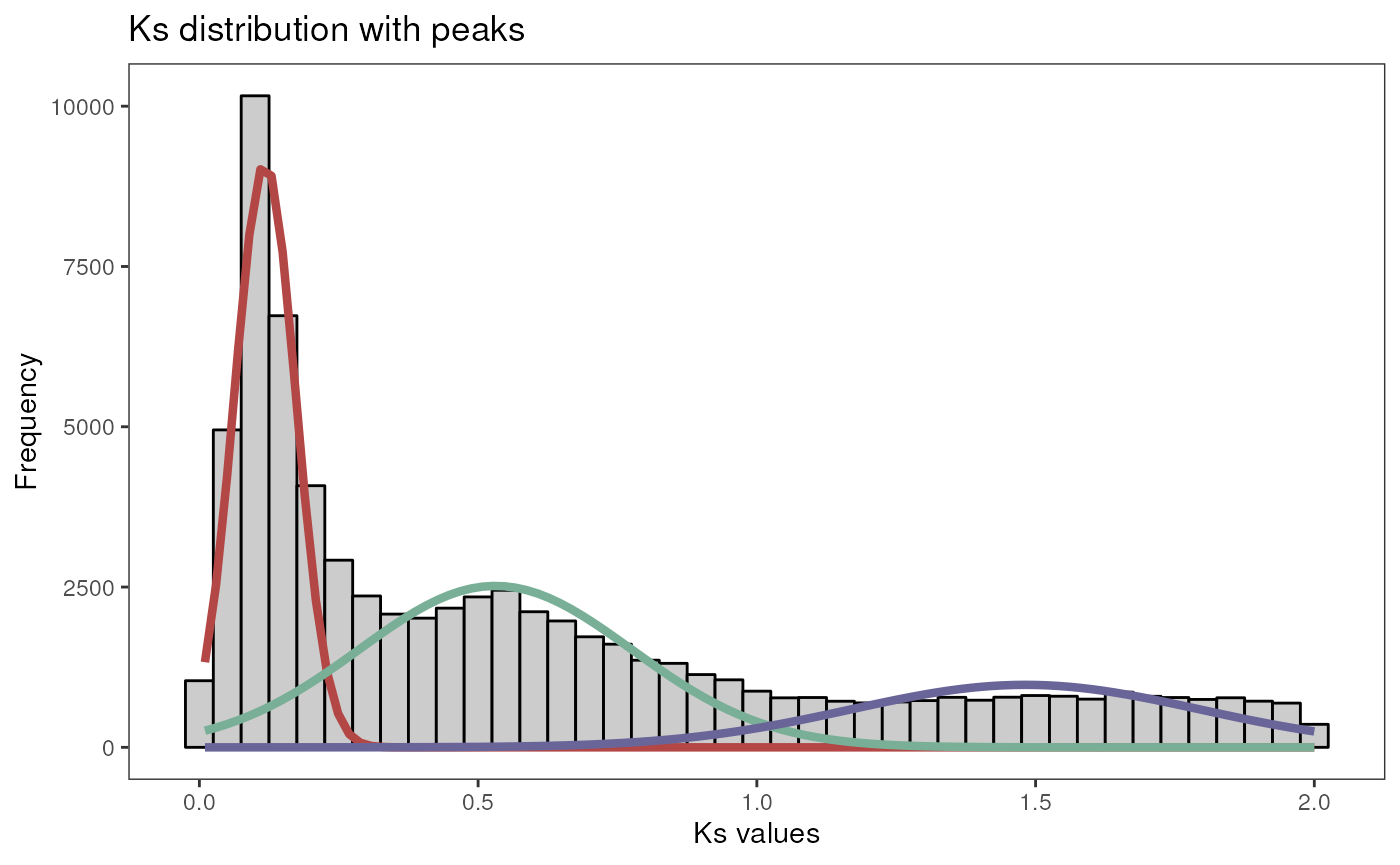

As we can see, the presence of 3 peaks is more supported (lowest BIC). The function returns a list with the mean, variance and amplitude of mixture components (i.e., peaks), as well as the $K_s$ distribution itself.

Now, suppose you just want to get the first 2 peaks. You can do that by explictly saying to find_ks_peaks() how many peaks there are.

# Find 2 peaks ignoring Ks values > 1
peaks <- find_ks_peaks(gmax_ks$Ks, npeaks = 2, max_ks = 1)
plot_ks_peaks(peaks)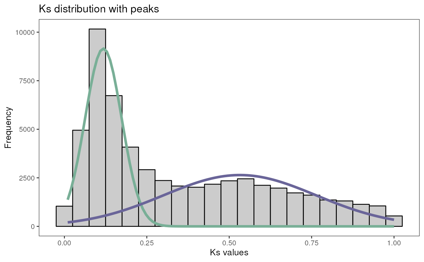

Important consideration on GMMs and $K_s$ distributions: Peaks identified with GMMs should not be blindly regarded as “the truth”. Using GMMs to find peaks in $K_s$ distributions can lead to problems such as overfitting and overclustering (Tiley, Barker, and Burleigh 2018). Some general recommendations are:

Use your prior knowledge. If you know how many peaks there are (e.g., based on literature evidence), just tell the number to find_ks_peaks(). Likewise, if you are not sure about how many peaks there are, but you know the maximum number of peaks is N, don’t test for the presence of >N peaks. GMMs can incorrectly identify more peaks than the actual number.
Test the significance of each peak with SiZer (Significant ZERo crossings of derivatives) maps (Chaudhuri and Marron 1999). This can be done with the function SiZer() from the R package feature.

As an example of a SiZer map, let’s use feature::SiZer() to assess the significance of the 2 peaks we found previously.

# Get numeric vector of Ks values <= 1
ks <- gmax_ks$Ks[gmax_ks$Ks <= 1]

# Get SiZer map
feature::SiZer(ks)
#> Warning: no DISPLAY variable so Tk is not available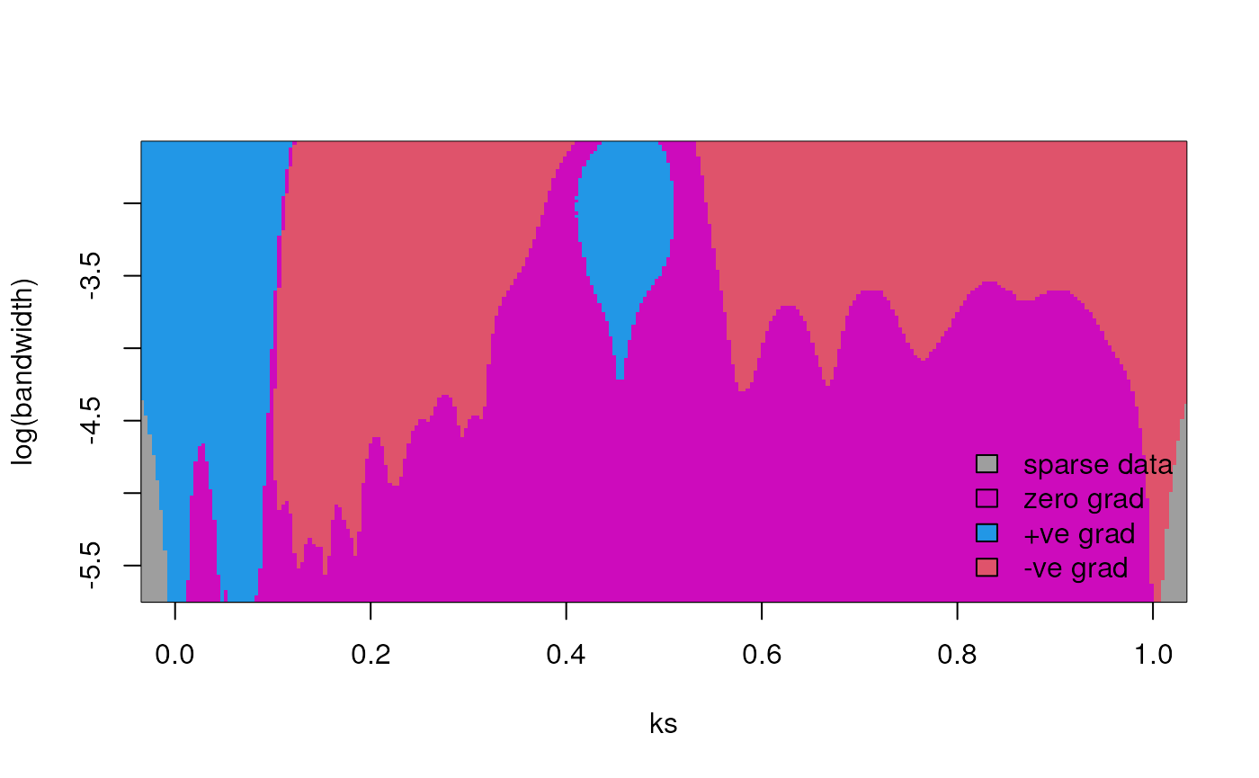

The blue regions in the SiZer map indicate significantly increasing regions of the curve, which support the 2 peaks we found.

Classifying genes by age groups

Finally, you can use the peaks you obtained before to classify gene pairs by age group. Age groups are defined based on the $K_s$ peak to which pairs belong. This is useful if you want to analyze duplicate pairs from a specific WGD event, for instance. You can do this with the function split_pairs_by_peak(). This function returns a list containing the classified pairs in a data frame, and a ggplot object with the age boundaries highlighted in the histogram of $K_s$ values.

# Gene pairs without age-based classification
head(gmax_ks)
#>              dup1            dup2     Ks type
#> 1 GLYMA_07G035600 GLYMA_16G004800 0.1670   SD
#> 2 GLYMA_18G275200 GLYMA_08G252600 0.1070   SD
#> 3 GLYMA_09G282200 GLYMA_20G003400 0.0822   SD
#> 4 GLYMA_01G166400 GLYMA_11G077000 0.0904   SD
#> 5 GLYMA_07G252100 GLYMA_17G022300 0.1400   SD
#> 6 GLYMA_05G133100 GLYMA_08G087600 0.0883   SD

# Classify gene pairs by age group
pairs_age_group <- split_pairs_by_peak(gmax_ks[, c(1,2,3)], peaks)

# Inspecting the output
names(pairs_age_group)
#> [1] "pairs" "plot"

# Take a look at the classified gene pairs
head(pairs_age_group$pairs)
#>              dup1            dup2     ks peak
#> 1 GLYMA_07G035600 GLYMA_16G004800 0.1670    1
#> 2 GLYMA_18G275200 GLYMA_08G252600 0.1070    1
#> 3 GLYMA_09G282200 GLYMA_20G003400 0.0822    1
#> 4 GLYMA_01G166400 GLYMA_11G077000 0.0904    1
#> 5 GLYMA_07G252100 GLYMA_17G022300 0.1400    1
#> 6 GLYMA_05G133100 GLYMA_08G087600 0.0883    1

# Visualize Ks distro with age boundaries
pairs_age_group$plot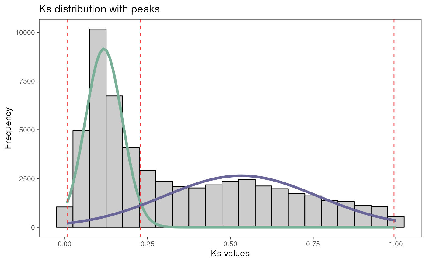

Age groups can also be used to identify SD gene pairs that likely originated from whole-genome duplications. The rationale here is that segmental duplicates with $K_s$ values near $K_s$ peaks (indicating WGD events) were likely created by such WGDs. In a similar logic, SD pairs with $K_s$ values that are too distant from $K_s$ peaks (e.g., >2 standard deviations away from the mean) were likely created by duplications of large genomic segments, but not duplications of the entire genome.

As an example, to find gene pairs in the soybean genome that likely originated from the WGD event shared by all legumes (at ~58 million years ago), you’d need to extract SD pairs in age group 2 using the following code:

# Get all pairs in age group 2
pairs_ag2 <- pairs_age_group$pairs[pairs_age_group$pairs$peak == 2, c(1,2)]

# Get all SD pairs
sd_pairs <- gmax_ks[gmax_ks$type == "SD", c(1,2)]

# Merge tables
pairs_wgd_legumes <- merge(pairs_ag2, sd_pairs)

head(pairs_wgd_legumes)
#>              dup1            dup2
#> 1 GLYMA_01G001800 GLYMA_07G130700
#> 2 GLYMA_01G002100 GLYMA_05G221300
#> 3 GLYMA_01G002300 GLYMA_07G130100
#> 4 GLYMA_01G002600 GLYMA_07G129700
#> 5 GLYMA_01G003500 GLYMA_05G222800
#> 6 GLYMA_01G003500 GLYMA_08G029700

Data visualization

Last but not least, doubletrouble provides users with graphical functions to produce publication-ready plots from the output of classify_gene_pairs(), classify_genes(), and pairs2kaks(). Let’s take a look at them one by one.

Visualizing the frequency of duplicates per mode

To visualize the frequency of duplicated gene pairs or genes by duplication type (as returned by classify_gene_pairs() and classify_genes(), respectively), you will first need to create a data frame of counts with duplicates2counts(). To demonstrate how this works, we will use an example data set with duplicate pairs for 3 fungi species (and substitution rates, which will be ignored by duplicates2counts()).

# Load data set with pre-computed duplicates for 3 fungi species
data(fungi_kaks)
names(fungi_kaks)
#> [1] "saccharomyces_cerevisiae"  "candida_glabrata"         
#> [3] "schizosaccharomyces_pombe"
head(fungi_kaks$saccharomyces_cerevisiae)
#>      dup1    dup2       Ka       Ks  Ka_Ks type
#> 1 YGR032W YLR342W 0.058800 5.240000 0.0112   SD
#> 2 YOR396W YPL283C 0.004010 0.009920 0.4040   SD
#> 3 YJL225C YIL177C 0.000253 0.000758 0.3340   SD
#> 4 YNR031C YCR073C 0.364000 5.070000 0.0718   SD
#> 5 YOR326W YAL029C 0.396000 5.150000 0.0769   SD
#> 6 YJL222W YIL173W 0.000276       NA     NA   SD

# Get a data frame of counts per mode in all species
counts_table <- duplicates2counts(fungi_kaks |> classify_genes())

counts_table
#>    type    n                   species
#> 1    SD  683  saccharomyces_cerevisiae
#> 2    TD   67  saccharomyces_cerevisiae
#> 3    PD   70  saccharomyces_cerevisiae
#> 4  rTRD    0  saccharomyces_cerevisiae
#> 5  dTRD    0  saccharomyces_cerevisiae
#> 6    DD 1790  saccharomyces_cerevisiae
#> 7    SD   14          candida_glabrata
#> 8    TD  104          candida_glabrata
#> 9    PD   42          candida_glabrata
#> 10 rTRD    0          candida_glabrata
#> 11 dTRD    0          candida_glabrata
#> 12   DD 1907          candida_glabrata
#> 13   SD   53 schizosaccharomyces_pombe
#> 14   TD   38 schizosaccharomyces_pombe
#> 15   PD   48 schizosaccharomyces_pombe
#> 16 rTRD    0 schizosaccharomyces_pombe
#> 17 dTRD    0 schizosaccharomyces_pombe
#> 18   DD 1853 schizosaccharomyces_pombe

Now, let’s visualize the frequency of duplicate gene pairs by duplication type with the function plot_duplicate_freqs(). You can visualize frequencies in three different ways, as demonstrated below.

# A) Facets
p1 <- plot_duplicate_freqs(counts_table)

# B) Stacked barplot, absolute frequencies
p2 <- plot_duplicate_freqs(counts_table, plot_type = "stack")

# C) Stacked barplot, relative frequencies
p3 <- plot_duplicate_freqs(counts_table, plot_type = "stack_percent")

# Combine plots, one per row
patchwork::wrap_plots(p1, p2, p3, nrow = 3) + 
    patchwork::plot_annotation(tag_levels = "A")

If you want to visually the frequency of duplicated genes (not gene pairs), you’d first need to classify genes into unique modes of duplication with classify_genes(), and then repeat the code above. For example:

# Frequency of duplicated genes by mode
classify_genes(fungi_kaks) |>   # classify genes into unique duplication types
    duplicates2counts() |>      # get a data frame of counts (long format)
    plot_duplicate_freqs()      # plot frequencies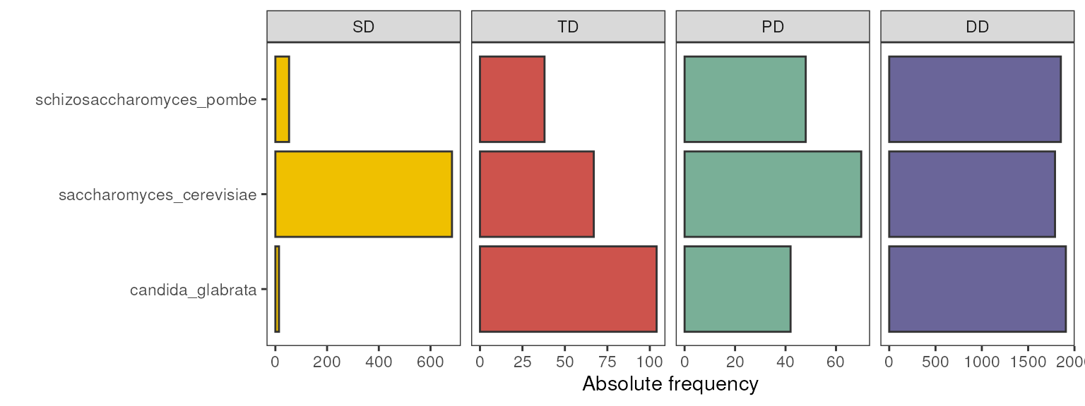

Visualizing $K_s$ distributions

As briefly demonstrated before, to plot a $K_s$ distribution for the whole paranome, you will use the function plot_ks_distro().

ks_df <- fungi_kaks$saccharomyces_cerevisiae

# A) Histogram, whole paranome
p1 <- plot_ks_distro(ks_df, plot_type = "histogram")

# B) Density, whole paranome
p2 <- plot_ks_distro(ks_df, plot_type = "density") 

# C) Histogram with density lines, whole paranome
p3 <- plot_ks_distro(ks_df, plot_type = "density_histogram")

# Combine plots side by side
patchwork::wrap_plots(p1, p2, p3, nrow = 1) +
    patchwork::plot_annotation(tag_levels = "A")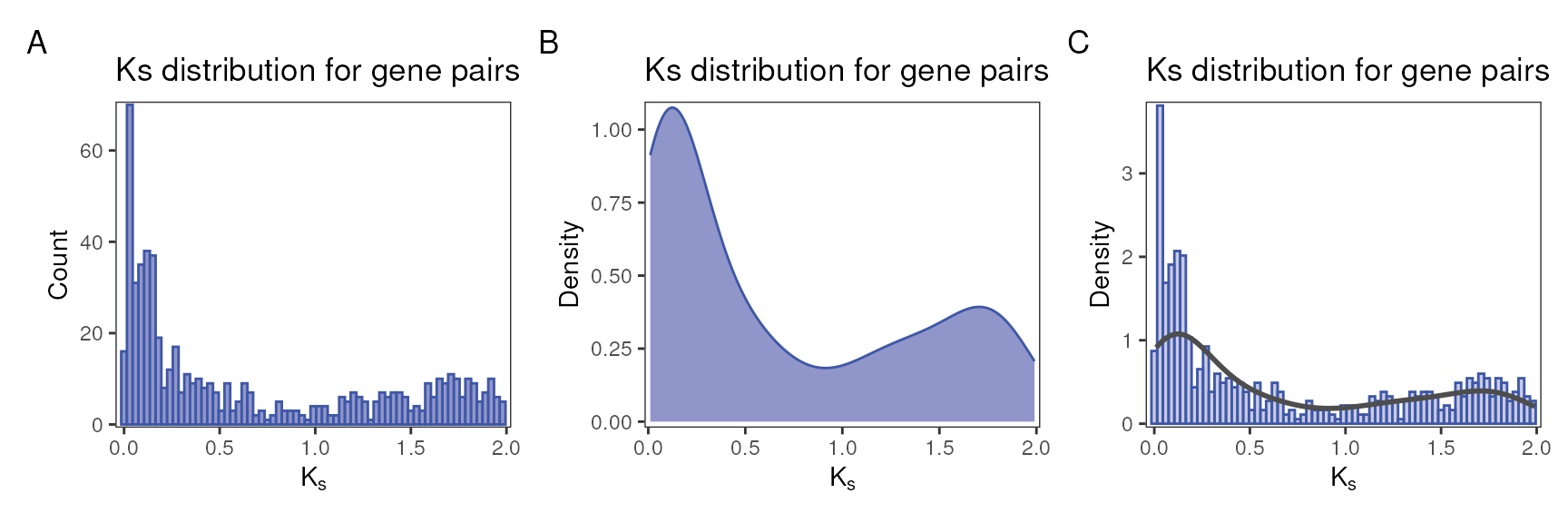

However, visualizing the distribution for the whole paranome can mask patterns that only happen for duplicates originating from particular duplication types. For instance, when looking for evidence of WGD events, visualizing the $K_s$ distribution for SD-derived pairs only can reveal whether syntenic genes cluster together, suggesting the presence of WGD history. To visualize the distribution by duplication type, use bytype = TRUE in plot_ks_distro().

# A) Duplicates by type, histogram
p1 <- plot_ks_distro(ks_df, bytype = TRUE, plot_type = "histogram")

# B) Duplicates by type, violin
p2 <- plot_ks_distro(ks_df, bytype = TRUE, plot_type = "violin")

# Combine plots side by side
patchwork::wrap_plots(p1, p2) +
    patchwork::plot_annotation(tag_levels = "A")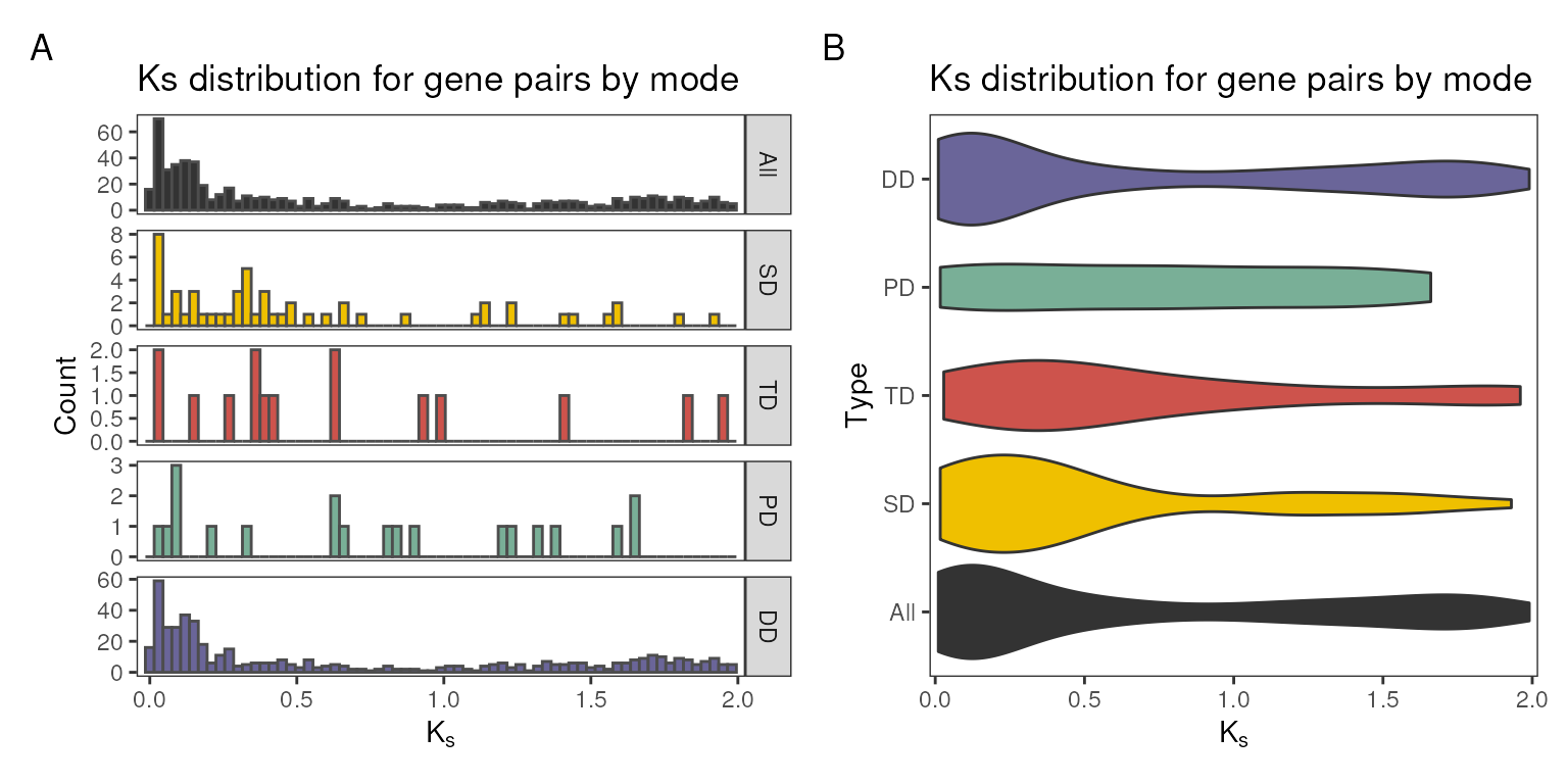

Visualizing substitution rates by species

The function plot_rates_by_species() can be used to show distributions of substitution rates ( $K_s$ , $K_a$ , or their ratio $K_a/K_s$ ) by species. You can choose which rate you want to visualize, and whether or not to group gene pairs by duplication mode, as demonstrated below.

# A) Ks for each species
p1 <- plot_rates_by_species(fungi_kaks)

# B) Ka/Ks by duplication type for each species
p2 <- plot_rates_by_species(fungi_kaks, rate_column = "Ka_Ks", bytype = TRUE)

# Combine plots - one per row
patchwork::wrap_plots(p1, p2, nrow = 2) +
    patchwork::plot_annotation(tag_levels = "A")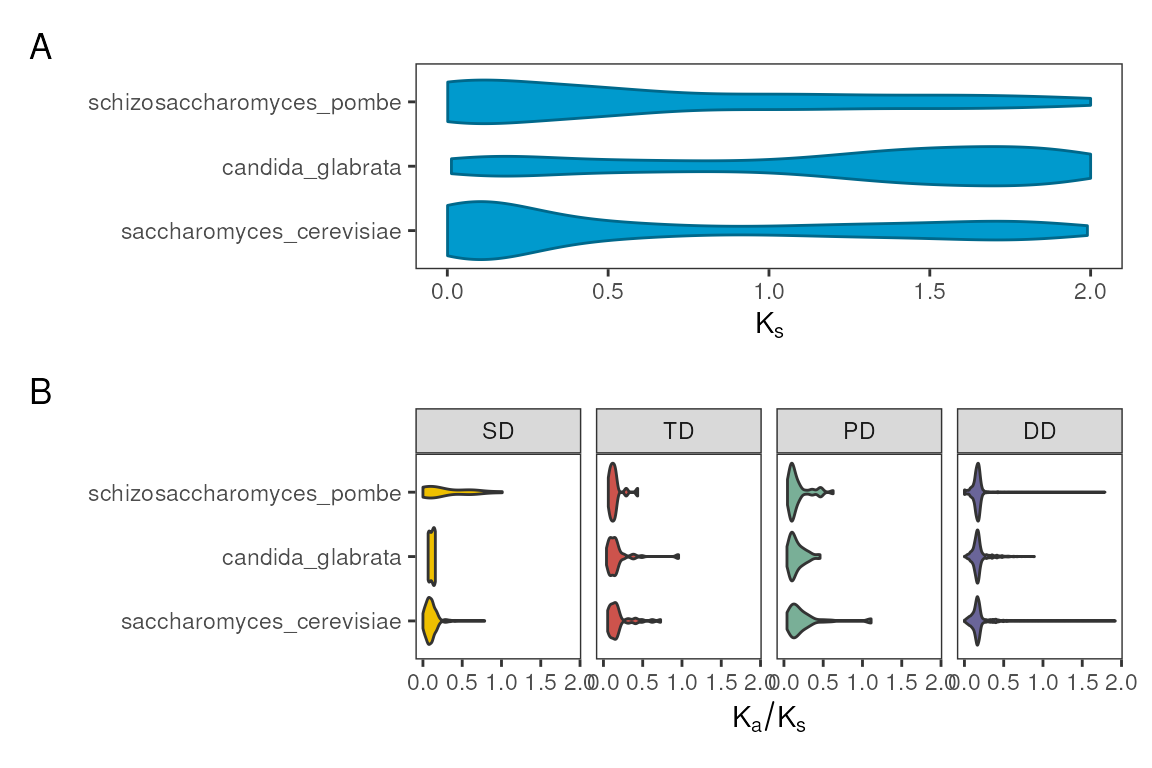

Session information

This document was created under the following conditions:

sessioninfo::session_info()
#> ─ Session info ───────────────────────────────────────────────────────────────
#>  setting  value
#>  version  R version 4.4.1 (2024-06-14)
#>  os       Ubuntu 22.04.5 LTS
#>  system   x86_64, linux-gnu
#>  ui       X11
#>  language en
#>  collate  en_US.UTF-8
#>  ctype    en_US.UTF-8
#>  tz       UTC
#>  date     2024-10-07
#>  pandoc   3.4 @ /usr/bin/ (via rmarkdown)
#> 
#> ─ Packages ───────────────────────────────────────────────────────────────────
#>  package              * version   date (UTC) lib source
#>  abind                  1.4-8     2024-09-12 [1] RSPM (R 4.4.0)
#>  ade4                   1.7-22    2023-02-06 [1] RSPM (R 4.4.0)
#>  AnnotationDbi        * 1.67.0    2024-05-01 [1] Bioconductor 3.20 (R 4.4.0)
#>  ape                    5.8       2024-04-11 [1] RSPM (R 4.4.0)
#>  Biobase              * 2.65.1    2024-08-28 [1] Bioconductor 3.20 (R 4.4.1)
#>  BiocFileCache          2.13.0    2024-05-01 [1] Bioconductor 3.20 (R 4.4.0)
#>  BiocGenerics         * 0.51.3    2024-10-02 [1] Bioconductor 3.20 (R 4.4.1)
#>  BiocIO                 1.15.2    2024-08-23 [1] Bioconductor 3.20 (R 4.4.1)
#>  BiocManager            1.30.25   2024-08-28 [2] CRAN (R 4.4.1)
#>  BiocParallel           1.39.0    2024-05-01 [1] Bioconductor 3.20 (R 4.4.0)
#>  BiocStyle            * 2.33.1    2024-06-12 [1] Bioconductor 3.20 (R 4.4.0)
#>  biomaRt                2.61.3    2024-08-06 [1] Bioconductor 3.20 (R 4.4.1)
#>  Biostrings             2.73.2    2024-09-26 [1] Bioconductor 3.20 (R 4.4.1)
#>  bit                    4.5.0     2024-09-20 [1] RSPM (R 4.4.0)
#>  bit64                  4.5.2     2024-09-22 [1] RSPM (R 4.4.0)
#>  bitops                 1.0-9     2024-10-03 [1] RSPM (R 4.4.0)
#>  blob                   1.2.4     2023-03-17 [1] RSPM (R 4.4.0)
#>  bookdown               0.40      2024-07-02 [1] RSPM (R 4.4.0)
#>  bslib                  0.8.0     2024-07-29 [2] RSPM (R 4.4.0)
#>  cachem                 1.1.0     2024-05-16 [2] RSPM (R 4.4.0)
#>  cli                    3.6.3     2024-06-21 [2] RSPM (R 4.4.0)
#>  coda                   0.19-4.1  2024-01-31 [1] RSPM (R 4.4.0)
#>  codetools              0.2-20    2024-03-31 [3] CRAN (R 4.4.1)
#>  colorspace             2.1-1     2024-07-26 [1] RSPM (R 4.4.0)
#>  crayon                 1.5.3     2024-06-20 [2] RSPM (R 4.4.0)
#>  curl                   5.2.3     2024-09-20 [2] RSPM (R 4.4.0)
#>  DBI                    1.2.3     2024-06-02 [1] RSPM (R 4.4.0)
#>  dbplyr                 2.5.0     2024-03-19 [1] RSPM (R 4.4.0)
#>  DelayedArray           0.31.14   2024-10-03 [1] Bioconductor 3.20 (R 4.4.1)
#>  desc                   1.4.3     2023-12-10 [2] RSPM (R 4.4.0)
#>  digest                 0.6.37    2024-08-19 [2] RSPM (R 4.4.0)
#>  doParallel             1.0.17    2022-02-07 [1] RSPM (R 4.4.0)
#>  doubletrouble        * 1.5.4     2024-10-07 [1] Bioconductor
#>  dplyr                  1.1.4     2023-11-17 [1] RSPM (R 4.4.0)
#>  evaluate               1.0.0     2024-09-17 [2] RSPM (R 4.4.0)
#>  fansi                  1.0.6     2023-12-08 [2] RSPM (R 4.4.0)
#>  farver                 2.1.2     2024-05-13 [1] RSPM (R 4.4.0)
#>  fastmap                1.2.0     2024-05-15 [2] RSPM (R 4.4.0)
#>  feature                1.2.15    2021-02-10 [1] RSPM (R 4.4.0)
#>  filelock               1.0.3     2023-12-11 [1] RSPM (R 4.4.0)
#>  foreach                1.5.2     2022-02-02 [1] RSPM (R 4.4.0)
#>  fs                     1.6.4     2024-04-25 [2] RSPM (R 4.4.0)
#>  generics               0.1.3     2022-07-05 [1] RSPM (R 4.4.0)
#>  GenomeInfoDb         * 1.41.2    2024-10-02 [1] Bioconductor 3.20 (R 4.4.1)
#>  GenomeInfoDbData       1.2.13    2024-10-02 [1] Bioconductor
#>  GenomicAlignments      1.41.0    2024-05-01 [1] Bioconductor 3.20 (R 4.4.0)
#>  GenomicFeatures      * 1.57.1    2024-09-27 [1] Bioconductor 3.20 (R 4.4.1)
#>  GenomicRanges        * 1.57.1    2024-06-12 [1] Bioconductor 3.20 (R 4.4.0)
#>  ggnetwork              0.5.13    2024-02-14 [1] RSPM (R 4.4.0)
#>  ggplot2                3.5.1     2024-04-23 [1] RSPM (R 4.4.0)
#>  glue                   1.8.0     2024-09-30 [2] RSPM (R 4.4.0)
#>  gtable                 0.3.5     2024-04-22 [1] RSPM (R 4.4.0)
#>  highr                  0.11      2024-05-26 [2] RSPM (R 4.4.0)
#>  hms                    1.1.3     2023-03-21 [1] RSPM (R 4.4.0)
#>  htmltools              0.5.8.1   2024-04-04 [2] RSPM (R 4.4.0)
#>  htmlwidgets            1.6.4     2023-12-06 [2] RSPM (R 4.4.0)
#>  httr                   1.4.7     2023-08-15 [1] RSPM (R 4.4.0)
#>  httr2                  1.0.5     2024-09-26 [2] RSPM (R 4.4.0)
#>  igraph                 2.0.3     2024-03-13 [1] RSPM (R 4.4.0)
#>  intergraph             2.0-4     2024-02-01 [1] RSPM (R 4.4.0)
#>  IRanges              * 2.39.2    2024-07-17 [1] Bioconductor 3.20 (R 4.4.1)
#>  iterators              1.0.14    2022-02-05 [1] RSPM (R 4.4.0)
#>  jquerylib              0.1.4     2021-04-26 [2] RSPM (R 4.4.0)
#>  jsonlite               1.8.9     2024-09-20 [2] RSPM (R 4.4.0)
#>  KEGGREST               1.45.1    2024-06-17 [1] Bioconductor 3.20 (R 4.4.0)
#>  KernSmooth             2.23-24   2024-05-17 [3] CRAN (R 4.4.1)
#>  knitr                  1.48      2024-07-07 [2] RSPM (R 4.4.0)
#>  ks                     1.14.3    2024-09-20 [1] RSPM (R 4.4.0)
#>  labeling               0.4.3     2023-08-29 [1] RSPM (R 4.4.0)
#>  lattice                0.22-6    2024-03-20 [3] CRAN (R 4.4.1)
#>  lifecycle              1.0.4     2023-11-07 [2] RSPM (R 4.4.0)
#>  magrittr               2.0.3     2022-03-30 [2] RSPM (R 4.4.0)
#>  MASS                   7.3-61    2024-06-13 [2] RSPM (R 4.4.0)
#>  Matrix                 1.7-0     2024-04-26 [3] CRAN (R 4.4.1)
#>  MatrixGenerics         1.17.0    2024-05-01 [1] Bioconductor 3.20 (R 4.4.0)
#>  matrixStats            1.4.1     2024-09-08 [1] RSPM (R 4.4.0)
#>  mclust                 6.1.1     2024-04-29 [1] RSPM (R 4.4.0)
#>  memoise                2.0.1     2021-11-26 [2] RSPM (R 4.4.0)
#>  MSA2dist               1.9.0     2024-05-01 [1] Bioconductor 3.20 (R 4.4.0)
#>  munsell                0.5.1     2024-04-01 [1] RSPM (R 4.4.0)
#>  mvtnorm                1.3-1     2024-09-03 [1] RSPM (R 4.4.0)
#>  network                1.18.2    2023-12-05 [1] RSPM (R 4.4.0)
#>  networkD3              0.4       2017-03-18 [1] RSPM (R 4.4.0)
#>  nlme                   3.1-166   2024-08-14 [2] RSPM (R 4.4.0)
#>  patchwork              1.3.0     2024-09-16 [1] RSPM (R 4.4.0)
#>  pheatmap               1.0.12    2019-01-04 [1] RSPM (R 4.4.0)
#>  pillar                 1.9.0     2023-03-22 [2] RSPM (R 4.4.0)
#>  pkgconfig              2.0.3     2019-09-22 [2] RSPM (R 4.4.0)
#>  pkgdown                2.1.1     2024-09-17 [2] RSPM (R 4.4.0)
#>  png                    0.1-8     2022-11-29 [1] RSPM (R 4.4.0)
#>  pracma                 2.4.4     2023-11-10 [1] RSPM (R 4.4.0)
#>  prettyunits            1.2.0     2023-09-24 [2] RSPM (R 4.4.0)
#>  progress               1.2.3     2023-12-06 [1] RSPM (R 4.4.0)
#>  purrr                  1.0.2     2023-08-10 [2] RSPM (R 4.4.0)
#>  pwalign                1.1.0     2024-05-01 [1] Bioconductor 3.20 (R 4.4.0)
#>  R6                     2.5.1     2021-08-19 [2] RSPM (R 4.4.0)
#>  ragg                   1.3.3     2024-09-11 [2] RSPM (R 4.4.0)
#>  rappdirs               0.3.3     2021-01-31 [2] RSPM (R 4.4.0)
#>  RColorBrewer           1.1-3     2022-04-03 [1] RSPM (R 4.4.0)
#>  Rcpp                   1.0.13    2024-07-17 [2] RSPM (R 4.4.0)
#>  RCurl                  1.98-1.16 2024-07-11 [1] RSPM (R 4.4.0)
#>  restfulr               0.0.15    2022-06-16 [1] RSPM (R 4.4.0)
#>  rjson                  0.2.23    2024-09-16 [1] RSPM (R 4.4.0)
#>  rlang                  1.1.4     2024-06-04 [2] RSPM (R 4.4.0)
#>  rmarkdown              2.28      2024-08-17 [2] RSPM (R 4.4.0)
#>  Rsamtools              2.21.2    2024-09-26 [1] Bioconductor 3.20 (R 4.4.1)
#>  RSQLite                2.3.7     2024-05-27 [1] RSPM (R 4.4.0)
#>  rtracklayer            1.65.0    2024-05-01 [1] Bioconductor 3.20 (R 4.4.0)
#>  S4Arrays               1.5.10    2024-09-29 [1] Bioconductor 3.20 (R 4.4.1)
#>  S4Vectors            * 0.43.2    2024-07-17 [1] Bioconductor 3.20 (R 4.4.1)
#>  sass                   0.4.9     2024-03-15 [2] RSPM (R 4.4.0)
#>  scales                 1.3.0     2023-11-28 [1] RSPM (R 4.4.0)
#>  seqinr                 4.2-36    2023-12-08 [1] RSPM (R 4.4.0)
#>  sessioninfo            1.2.2     2021-12-06 [2] RSPM (R 4.4.0)
#>  SparseArray            1.5.43    2024-10-04 [1] Bioconductor 3.20 (R 4.4.1)
#>  statnet.common         4.10.0    2024-10-06 [1] RSPM (R 4.4.0)
#>  stringi                1.8.4     2024-05-06 [2] RSPM (R 4.4.0)
#>  stringr                1.5.1     2023-11-14 [2] RSPM (R 4.4.0)
#>  SummarizedExperiment   1.35.3    2024-10-02 [1] Bioconductor 3.20 (R 4.4.1)
#>  syntenet             * 1.7.0     2024-05-01 [1] Bioconductor 3.20 (R 4.4.0)
#>  systemfonts            1.1.0     2024-05-15 [2] RSPM (R 4.4.0)
#>  textshaping            0.4.0     2024-05-24 [2] RSPM (R 4.4.0)
#>  tibble                 3.2.1     2023-03-20 [2] RSPM (R 4.4.0)
#>  tidyr                  1.3.1     2024-01-24 [1] RSPM (R 4.4.0)
#>  tidyselect             1.2.1     2024-03-11 [1] RSPM (R 4.4.0)
#>  txdbmaker            * 1.1.1     2024-06-20 [1] Bioconductor 3.20 (R 4.4.0)
#>  UCSC.utils             1.1.0     2024-05-01 [1] Bioconductor 3.20 (R 4.4.0)
#>  utf8                   1.2.4     2023-10-22 [2] RSPM (R 4.4.0)
#>  vctrs                  0.6.5     2023-12-01 [2] RSPM (R 4.4.0)
#>  withr                  3.0.1     2024-07-31 [2] RSPM (R 4.4.0)
#>  xfun                   0.48      2024-10-03 [2] RSPM (R 4.4.0)
#>  XML                    3.99-0.17 2024-06-25 [1] RSPM (R 4.4.0)
#>  xml2                   1.3.6     2023-12-04 [2] RSPM (R 4.4.0)
#>  XVector                0.45.0    2024-05-01 [1] Bioconductor 3.20 (R 4.4.0)
#>  yaml                   2.3.10    2024-07-26 [2] RSPM (R 4.4.0)
#>  zlibbioc               1.51.1    2024-06-05 [1] Bioconductor 3.20 (R 4.4.0)
#> 
#>  [1] /__w/_temp/Library
#>  [2] /usr/local/lib/R/site-library
#>  [3] /usr/local/lib/R/library
#> 
#> ──────────────────────────────────────────────────────────────────────────────

References

Chaudhuri, Probal, and James S Marron. 1999. “SiZer for Exploration of Structures in Curves.” Journal of the American Statistical Association 94 (447): 807–23.

Ohno, Susumu. 2013. Evolution by Gene Duplication. Springer Science & Business Media.

Schmutz, Jeremy, Steven B Cannon, Jessica Schlueter, Jianxin Ma, Therese Mitros, William Nelson, David L Hyten, et al. 2010. “Genome Sequence of the Palaeopolyploid Soybean.” Nature 463 (7278): 178–83.

Tiley, George P, Michael S Barker, and J Gordon Burleigh. 2018. “Assessing the Performance of Ks Plots for Detecting Ancient Whole Genome Duplications.” Genome Biology and Evolution 10 (11): 2882–98.

Vanneste, Kevin, Yves Van de Peer, and Steven Maere. 2013. “Inference of Genome Duplications from Age Distributions Revisited.” Molecular Biology and Evolution 30 (1): 177–90.

Wang, Dapeng, Yubin Zhang, Zhang Zhang, Jiang Zhu, and Jun Yu. 2010. “KaKs_calculator 2.0: A Toolkit Incorporating Gamma-Series Methods and Sliding Window Strategies.” Genomics, Proteomics & Bioinformatics 8 (1): 77–80.

Yates, Andrew D, James Allen, Ridwan M Amode, Andrey G Azov, Matthieu Barba, Andrés Becerra, Jyothish Bhai, et al. 2022. “Ensembl Genomes 2022: An Expanding Genome Resource for Non-Vertebrates.” Nucleic Acids Research 50 (D1): D996–1003.

Fabricio Almeida-Silva

Yves Van de Peer