2  Dealing with multiple data sets: consensus modules and module preservation

In this lesson, you will learn how to compare coexpression networks to identify preserved modules. At the end of the lesson, you will be able to:

• understand the concept of and identify consensus modules across data sets
• associate consensus modules to traits
• calculate module preservation statistics

Let’s start by loading the packages we will use.

set.seed(123) # for reproducibility

# Load required packages
library(tidyverse)
library(BioNERO)
library(SummarizedExperiment)
library(here)

2.1 Getting to know the example data

In this chapter, we will use gene expression data from two BioProjects:

1. PRJNA800609: soybean pods infected with the fungus Colletotrichum truncatum. Original data generated by Zhu et al. (2022).

2. PRJNA574764: soybean roots infected with the oomycete Phytophthora sojae. Original data generated by Ronne et al. (2020).

Our goal here is to explore similarities and differences in expression profiles between these two data sets.

Data are available as .rda files in the data/ directory of the GitHub repo associated with this course, and they were downloaded from The Soybean Expression Atlas v2 (Almeida-Silva, Pedrosa-Silva, and Venancio 2023) by searching by BioProject IDs. These .rda files contain SummarizedExperiment objects that store gene expression data and sample metadata.

Let’s load the data and explore them briefly.

# Load expression data
load(here("data", "se_PRJNA800609.rda"))
load(here("data", "se_PRJNA574764.rda"))

# Rename object to a simpler name
exp1 <- se_PRJNA800609
exp2 <- se_PRJNA574764

rm(se_PRJNA800609)
rm(se_PRJNA574764)

# Take a look at the object
exp1

class: SummarizedExperiment 
dim: 31422 60 
metadata(0):
assays(1): ''
rownames(31422): Glyma.15G153300 Glyma.15G153400 ... Glyma.09G145600
  Glyma.09G145700
rowData names(0):
colnames(60): SAMN25263487 SAMN25263488 ... SAMN25263525 SAMN25263526
colData names(4): Part Cultivar Treatment Timepoint

exp2

class: SummarizedExperiment 
dim: 32674 49 
metadata(0):
assays(1): ''
rownames(32674): Glyma.06G124400 Glyma.06G124500 ... Glyma.19G260900
  Glyma.19G261200
rowData names(0):
colnames(49): SAMN12868627 SAMN12868668 ... SAMN12868625 SAMN12868626
colData names(4): Part Cultivar Treatment Timepoint

colData(exp1)

DataFrame with 60 rows and 4 columns
                    Part     Cultivar   Treatment   Timepoint
             <character>  <character> <character> <character>
SAMN25263487         pod         ZC-2     control          8h
SAMN25263488         pod         ZC-2     control          8h
SAMN25263507         pod         ZC-2    infected         48h
SAMN25263508         pod         ZC-2    infected         48h
SAMN25263527         pod Zhechun NO.3    infected         12h
...                  ...          ...         ...         ...
SAMN25263522         pod Zhechun NO.3     control         12h
SAMN25263523         pod Zhechun NO.3     control         12h
SAMN25263524         pod Zhechun NO.3     control         12h
SAMN25263525         pod Zhechun NO.3    infected         12h
SAMN25263526         pod Zhechun NO.3    infected         12h

colData(exp2)

DataFrame with 49 rows and 4 columns
                    Part    Cultivar   Treatment   Timepoint
             <character> <character> <character> <character>
SAMN12868627        root       Misty    infected       4 dpi
SAMN12868668        root   PI 449459    infected      14 dpi
SAMN12868669        root   PI 449459    infected      14 dpi
SAMN12868649        root   PI 449459     control       0 dpi
SAMN12868628        root       Misty    infected       7 dpi
...                  ...         ...         ...         ...
SAMN12868647        root   PI 449459     control       0 dpi
SAMN12868648        root   PI 449459     control       0 dpi
SAMN12868624        root       Misty     control       0 dpi
SAMN12868625        root       Misty    infected       4 dpi
SAMN12868626        root       Misty    infected       4 dpi

Practice

1. Explore the sample metadata of exp1 and exp2 and answer the questions below:

• How many different cultivars are there?
• What are the levels of the Treatment variable, and how many samples are there for each level?
• How many samples are there for each timepoint?

Show me the solutions

# Question 1: # of cultivars
length(unique(exp1$Cultivar))

[1] 2

length(unique(exp2$Cultivar))

[1] 2

# Question 2: levels of the `Treatment` variable
table(exp1$Treatment)

 control infected 
      30       30 

table(exp2$Treatment)

 control infected 
       6       43 

# Question 3: # of samples for each timepoint
table(exp1$Timepoint)

12h 24h 48h  4h  8h 
 12  12  12  12  12 

table(exp2$Timepoint)

 0 dpi 14 dpi 21 dpi  4 dpi  7 dpi 
     6     12      8     12     11 

2.2 Data preprocessing

Now, we will preprocess the two data sets using the same parameters with exp_preprocess(). In details, we will:

1. Keep only genes with median TPM >=5.
2. Keep only the top 10k genes with the highest variances.

# Store each expression data in a list, each data set in a list element
1exp_list <- list(
    colletrotrichum_infection = exp1,
    phytophthora_infection = exp2
)

# Loop through the list and preprocess data
2exp_list <- lapply(
    exp_list,
3    exp_preprocess,
4    min_exp = 5, variance_filter = TRUE, n = 1e4, Zk_filtering = FALSE
)

# Keep only genes that are shared between the two sets
shared <- intersect(
    rownames(exp_list$colletrotrichum_infection),
    rownames(exp_list$phytophthora_infection)
)

exp_list <- lapply(exp_list, function(x) x[shared, ])

1

Store each expression data set in a list element.

2

Loop through each element of the list exp_list, and

3

execute the function exp_preprocess,

4

using these parameters.

Now, we have a list of processed expression data. This list, with each element representing a different data set, is what we will use for all network comparison functions in the next sections.

Practice

1. How many genes and samples are there in each processed data?

2. If we selected the top 10k genes with the highest variances, why do we not have 10k genes in each final set?

Show me the solutions

# Q1
sapply(exp_list, nrow)

colletrotrichum_infection    phytophthora_infection 
                     5530                      5530 

sapply(exp_list, ncol)

colletrotrichum_infection    phytophthora_infection 
                       60                        49 

#' Q2: the genes with the highest variances are not the same in both sets.
#' Thus, when filtering the data to keep only shared genes, some genes are
#' removed.

2.3 Identifying and analyzing consensus modules

Consensus modules are coexpression modules present in different, independent data sets, and they can used to find robust modules across data sets that study the same (or similar) conditions.

To identify them, BioNERO infers a GCN for each data set and looks for groups of genes that are densely connected in all data sets. Thus, the workflow here will be very similar to what we did in the previous lesson. We will:

1. Identify the optimal \(\beta\) power to which correlations will be raised (see previous chapter for more details on why this is done), but for each individual data set - consensus_SFT_fit()
2. Infer GCNs and identify consensus modules - consensus_modules().

Let’s obtain the \(\beta\) powers.

# Identify the optimal beta power for each data set
sfts <- consensus_SFT_fit(
    exp_list = exp_list,
    setLabels = names(exp_list),
    cor_method = "pearson"
)

   Power SFT.R.sq  slope truncated.R.sq mean.k. median.k. max.k.
1      5    0.924 -0.968          0.935   170.0    110.00    692
2      6    0.925 -1.050          0.936   127.0     75.40    589
3      7    0.923 -1.120          0.936    97.4     52.70    509
4      8    0.927 -1.160          0.944    76.5     37.10    445
5      9    0.928 -1.200          0.946    61.2     27.00    392
6     10    0.927 -1.230          0.947    49.7     19.80    349
7     11    0.929 -1.260          0.950    40.9     14.80    312
8     12    0.931 -1.290          0.954    34.0     11.10    281
9     13    0.940 -1.300          0.963    28.6      8.52    254
10    14    0.944 -1.320          0.968    24.2      6.55    231
11    15    0.948 -1.330          0.970    20.7      5.18    210
12    16    0.950 -1.340          0.973    17.8      4.03    192
13    17    0.954 -1.350          0.977    15.4      3.18    177
14    18    0.959 -1.350          0.982    13.4      2.51    163
15    19    0.960 -1.370          0.984    11.7      2.03    151
16    20    0.959 -1.380          0.985    10.3      1.64    140
   Power SFT.R.sq  slope truncated.R.sq mean.k. median.k. max.k.
1      5    0.866 -0.895          0.933  157.00    110.00    572
2      6    0.875 -1.000          0.942  116.00     71.10    493
3      7    0.874 -1.080          0.941   88.20     47.40    432
4      8    0.874 -1.140          0.936   68.90     32.40    382
5      9    0.844 -1.210          0.908   55.00     22.60    342
6     10    0.834 -1.260          0.893   44.70     16.10    308
7     11    0.828 -1.310          0.884   36.80     11.60    279
8     12    0.821 -1.340          0.875   30.70      8.48    255
9     13    0.785 -1.390          0.845   25.80      6.32    233
10    14    0.777 -1.420          0.843   22.00      4.77    215
11    15    0.791 -1.420          0.853   18.90      3.63    198
12    16    0.803 -1.420          0.863   16.30      2.79    184
13    17    0.813 -1.430          0.870   14.20      2.17    171
14    18    0.825 -1.430          0.882   12.40      1.69    159
15    19    0.800 -1.470          0.866   10.90      1.34    148
16    20    0.807 -1.460          0.874    9.66      1.06    139

sfts$power

colletrotrichum_infection    phytophthora_infection 
                        5                         5 

sfts$plot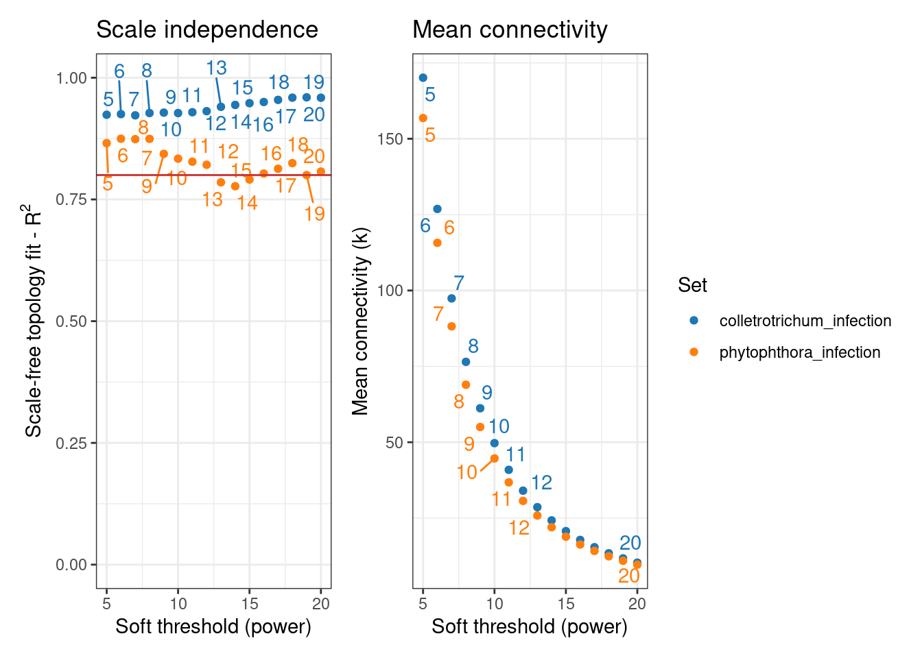

Next, let’s find consensus modules.

# Find consensus modules
consensus <- consensus_modules(
    exp_list, 
    power = sfts$power,
    cor_method = "pearson"
)

..connectivity..
..matrix multiplication (system BLAS)..
..normalization..
..done.
..connectivity..
..matrix multiplication (system BLAS)..
..normalization..
..done.
 ..done.
 multiSetMEs: Calculating module MEs.
   Working on set 1 ...
   Working on set 2 ...

# Taking a look at the consensus modules
plot_dendro_and_colors(consensus)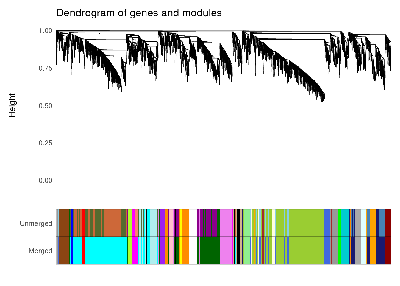

# Inspecting the output
names(consensus)

[1] "consMEs"             "exprSize"            "sampleInfo"         
[4] "genes_cmodules"      "dendro_plot_objects"

As you may have noticed, the output of consensus_modules() is very similar to the output of exp2gcn(). The output object is a list containing the following elements:

1. consMEs: list with consensus module eigengenes.
2. exprSize: list with number of data sets, and number of genes and samples for each set.
3. sampleInfo: list of data frames with sample metadata.
4. genes_cmodules: data frame with genes and their corresponding consensus modules.
5. dendro_plot_objects: objects for plotting with plot_dendro_and_colors().

Practice

Explore the output of consensus_modules() and answer the following questions:

1. How many consensus modules were identified between the two data sets?
2. What are the largest and the smallest consensus modules?
3. What is the mean and median number of genes per consensus modules?

Show me the solutions

# Q1
length(unique(consensus$genes_cmodules$Cons_modules))

[1] 30

# Q2
sort(table(consensus$genes_cmodules$Cons_modules))

         grey          blue         brown        yellow         green 
            8            34            38            54            57 
          red         black          pink        purple   greenyellow 
           61            66            68            75            77 
          tan        grey60     lightcyan    lightgreen   lightyellow 
           78            96            96            97            97 
      darkred darkturquoise      darkgrey        orange    darkorange 
          104           118           119           124           139 
        white       magenta   saddlebrown paleturquoise     royalblue 
          140           150           169           213           269 
       violet  midnightblue     darkgreen   yellowgreen          cyan 
          280           303           473           942           985 

# Q3
mean(table(consensus$genes_cmodules$Cons_modules))

[1] 184.3333

median(table(consensus$genes_cmodules$Cons_modules))

[1] 100.5

Next, you’d want to find correlations between consensus modules and traits of interest. Here, we will look for associations between consensus modules and the Treatment variable. Biologically speaking, we’re looking for shared transcriptional responses during infection with Colletotrichum truncatum and Phytophthora sojae (i.e., core immunity-related coexpression modules).

# Correlate consensus modules to traits
consensus_trait <- consensus_trait_cor(
    consensus,
    metadata_cols = "Treatment"
)

# Taking a look at the output
head(consensus_trait)

    trait              ME         cor     pvalue     group
1 control         MEblack          NA         NA Treatment
2 control       MEdarkred  0.26015095 0.07092879 Treatment
3 control          MEblue -0.14934335 0.30747782 Treatment
4 control MEdarkturquoise  0.18536193 0.20341269 Treatment
5 control         MEbrown          NA         NA Treatment
6 control         MEgreen  0.05251631 0.69147472 Treatment

# Plot consensus module-trait correlations
plot_module_trait_cor(consensus_trait)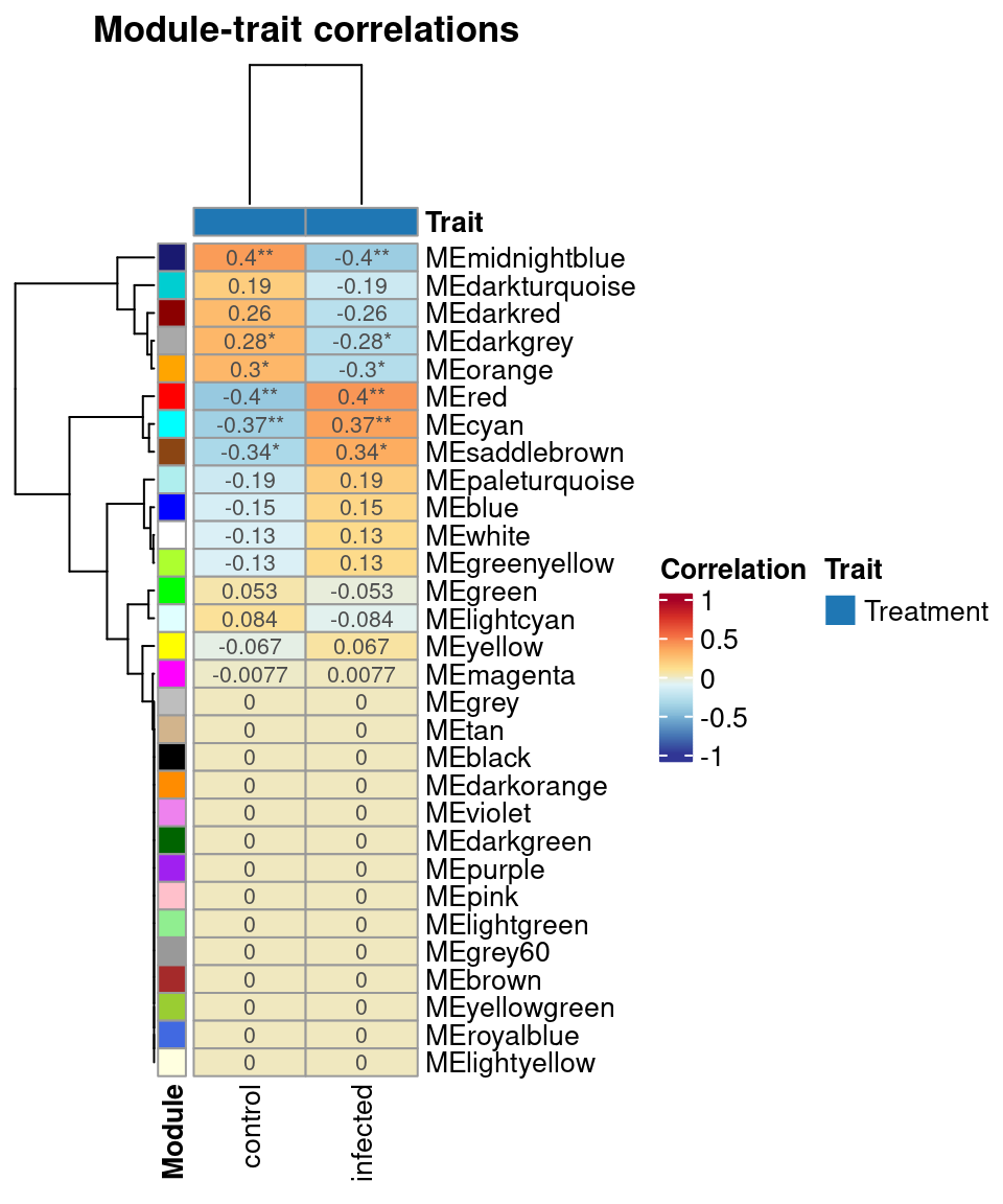

Practice

Explore the output of consensus_trait_cor() and answer the questions below:

1. Which consensus module has the highest positive correlation to the infected status of the Treatment variable?

2. Which consensus module has the highest negative correlation to the infected status of the Treatment variable?

3. (Advanced) Based on your biological knowledge, what gene functions would you expect to find in the modules you found in questions 1 and 2?

Show me the solutions

# Q1
cor_infected <- consensus_trait[consensus_trait$trait == "infected", ]
cor_infected[which.max(cor_infected$cor), ]

      trait    ME       cor      pvalue     group
59 infected MEred 0.4029435 0.003765978 Treatment

# Q2
cor_infected[which.min(cor_infected$cor), ]

      trait             ME        cor      pvalue     group
49 infected MEmidnightblue -0.3966709 0.004420417 Treatment

Challenge

Use the function module_enrichment() to perform a functional enrichment analysis for each consensus module. Then, try to interpret the results in light of the consensus module-trait associations you found previously.

Tip: to load the functional annotation data, use the following:

load(here("data", "gma_annotation.rda"))

Show me the solutions

# Load functional annotation data
load(here("data", "gma_annotation.rda"))

# Define background
background <- rownames(exp_list$colletrotrichum_infection)
    
# Perform the enrichment analysis
sim_net <- consensus
names(sim_net)[4] <- "genes_and_modules"
names(sim_net$genes_and_modules) <- c("Genes", "Modules")

enrich_mapman <- module_enrichment(sim_net, background, gma_annotation$MapMan)
enrich_interpro <- module_enrichment(sim_net, background, gma_annotation$InterPro)

2.4 Calculating module preservation statistics

When we infer consensus modules across data sets, we only consider shared modules, but we have no information on which modules are not shared between different data sets.

If you want to have a more detailed picture of which modules are preserved and which are not, you’d need to infer a separate network for each data set, and then calculate module preservation statistics between the networks.

Here, we will demonstrate how to do that using the same data set from the previous section. Since, we already have the processed data, we will proceed to GCN inference using the functions SFT_fit() and exp2gcn(), as we saw in Chapter 1.

# Get optimal beta power for each data set
powers <- lapply(exp_list, SFT_fit, cor_method = "pearson")

   Power SFT.R.sq  slope truncated.R.sq mean.k. median.k. max.k.
1      3    0.234 -0.774         0.0153  1130.0     997.0   1810
2      4    0.372 -0.725         0.2440   805.0     699.0   1510
3      5    0.530 -0.728         0.4860   602.0     509.0   1290
4      6    0.654 -0.757         0.6480   466.0     382.0   1130
5      7    0.767 -0.816         0.7850   372.0     295.0   1000
6      8    0.840 -0.872         0.8600   303.0     233.0    898
7      9    0.884 -0.923         0.9010   251.0     186.0    813
8     10    0.901 -0.968         0.9190   211.0     151.0    742
9     11    0.912 -1.010         0.9280   179.0     123.0    681
10    12    0.920 -1.050         0.9380   154.0     101.0    628
11    13    0.921 -1.080         0.9390   134.0      84.5    582
12    14    0.914 -1.110         0.9310   117.0      70.4    541
13    15    0.919 -1.140         0.9390   102.0      59.5    504
14    16    0.921 -1.160         0.9410    90.5      50.5    471
15    17    0.923 -1.180         0.9420    80.4      42.9    441
16    18    0.925 -1.200         0.9460    71.7      36.3    415
17    19    0.927 -1.220         0.9480    64.3      30.9    390
18    20    0.931 -1.240         0.9520    57.8      26.7    368
   Power SFT.R.sq   slope truncated.R.sq mean.k. median.k. max.k.
1      3  0.66100  4.4900          0.947  1140.0    1140.0   1510
2      4  0.44400  2.0600          0.883   803.0     797.0   1230
3      5  0.16500  0.6540          0.685   594.0     580.0   1050
4      6  0.00224 -0.0438          0.585   456.0     432.0    921
5      7  0.28100 -0.4140          0.709   359.0     330.0    818
6      8  0.64700 -0.6550          0.878   290.0     255.0    735
7      9  0.78900 -0.7960          0.926   238.0     199.0    669
8     10  0.82900 -0.8870          0.937   198.0     158.0    613
9     11  0.84100 -0.9530          0.933   168.0     126.0    566
10    12  0.85100 -1.0100          0.937   143.0     103.0    524
11    13  0.86000 -1.0500          0.943   123.0      83.2    488
12    14  0.86000 -1.0900          0.941   107.0      68.1    456
13    15  0.86100 -1.1200          0.940    93.7      56.2    428
14    16  0.85800 -1.1600          0.934    82.5      46.5    402
15    17  0.86800 -1.1700          0.939    73.0      38.7    379
16    18  0.85500 -1.2100          0.925    65.0      32.4    359
17    19  0.83400 -1.2400          0.905    58.2      27.2    340
18    20  0.83600 -1.2600          0.905    52.3      23.1    322

# Infer GCN for each data set
gcns <- lapply(seq_along(powers), function(n) {
    
    gcn <- exp2gcn(
        exp_list[[n]], 
        SFTpower = powers[[n]]$power, 
        cor_method = "pearson"
    )
    
    return(gcn)
})

..connectivity..
..matrix multiplication (system BLAS)..
..normalization..
..done.
..connectivity..
..matrix multiplication (system BLAS)..
..normalization..
..done.

Practice

How many modules are there in each network?

Show me the solutions

sapply(gcns, function(x) length(unique(x$genes_and_modules$Modules)))

[1] 12 17

Next, we can calculate module preservation statistics using the permutation-based approach implemented in NetRep.

# Calculate module preservation statistics
pres_netrep <- module_preservation(
    exp_list, 
    ref_net = gcns[[1]], 
    test_net = gcns[[2]], 
    algorithm = "netrep"
)

[2023-08-24 09:56:26 CEST] Validating user input...
[2023-08-24 09:56:26 CEST]   Checking matrices for problems...
[2023-08-24 09:56:28 CEST] Input ok!
[2023-08-24 09:56:28 CEST] Calculating preservation of network subsets from
                           dataset "colletrotrichum_infection" in dataset
                           "phytophthora_infection".
[2023-08-24 09:56:28 CEST]   Pre-computing network properties in dataset
                             "colletrotrichum_infection"...
[2023-08-24 09:56:29 CEST]   Calculating observed test statistics...
[2023-08-24 09:56:29 CEST]   Generating null distributions from 1000
                             permutations using 1 thread...


    0% completed.
    1% completed.
    2% completed.
    2% completed.
    3% completed.
    4% completed.
    5% completed.
    5% completed.
    6% completed.
    7% completed.
    8% completed.
    9% completed.
    9% completed.
   10% completed.
   11% completed.
   12% completed.
   13% completed.
   13% completed.
   14% completed.
   15% completed.
   16% completed.
   16% completed.
   17% completed.
   18% completed.
   19% completed.
   20% completed.
   20% completed.
   21% completed.
   22% completed.
   23% completed.
   24% completed.
   24% completed.
   25% completed.
   26% completed.
   27% completed.
   28% completed.
   28% completed.
   29% completed.
   30% completed.
   31% completed.
   31% completed.
   32% completed.
   33% completed.
   34% completed.
   35% completed.
   35% completed.
   36% completed.
   37% completed.
   38% completed.
   39% completed.
   39% completed.
   40% completed.
   41% completed.
   42% completed.
   42% completed.
   43% completed.
   44% completed.
   45% completed.
   46% completed.
   46% completed.
   47% completed.
   48% completed.
   49% completed.
   50% completed.
   50% completed.
   51% completed.
   52% completed.
   53% completed.
   54% completed.
   54% completed.
   55% completed.
   56% completed.
   57% completed.
   57% completed.
   58% completed.
   59% completed.
   60% completed.
   61% completed.
   61% completed.
   62% completed.
   63% completed.
   64% completed.
   64% completed.
   65% completed.
   66% completed.
   67% completed.
   68% completed.
   68% completed.
   69% completed.
   70% completed.
   71% completed.
   72% completed.
   72% completed.
   73% completed.
   74% completed.
   75% completed.
   75% completed.
   76% completed.
   77% completed.
   78% completed.
   79% completed.
   79% completed.
   80% completed.
   81% completed.
   82% completed.
   83% completed.
   83% completed.
   84% completed.
   85% completed.
   86% completed.
   87% completed.
   87% completed.
   88% completed.
   89% completed.
   90% completed.
   90% completed.
   91% completed.
   92% completed.
   93% completed.
   94% completed.
   94% completed.
   95% completed.
   96% completed.
   97% completed.
   98% completed.
   98% completed.
   99% completed.
  100% completed.
  100% completed.

[2023-08-24 09:58:37 CEST]   Calculating P-values...
[2023-08-24 09:58:38 CEST]   Collating results...
[2023-08-24 09:58:39 CEST] Done!

# Taking a look at the P-values for preservation statistics for each module
head(pres_netrep$p.values)

           avg.weight   coherence     cor.cor  cor.degree cor.contrib
black     0.000999001 0.000999001 0.000999001 0.000999001 0.000999001
blue      0.142857143 0.262737263 0.000999001 0.000999001 0.096903097
cyan      0.994005994 0.999000999 0.000999001 0.000999001 0.000999001
darkgreen 0.976023976 1.000000000 0.000999001 0.001998002 0.994005994
green     0.002997003 1.000000000 0.000999001 0.000999001 0.000999001
grey      0.986013986 1.000000000 0.001998002 0.176823177 0.138861139
              avg.cor avg.contrib
black     0.000999001 0.000999001
blue      0.000999001 0.188811189
cyan      0.000999001 0.000999001
darkgreen 0.000999001 0.100899101
green     0.000999001 0.000999001
grey      0.005994006 0.544455544

Note that, to calculate module preservation statistics, you always need to choose a reference network and a test network. Thus, the function module_preservation() will return which modules of the reference network that are preserved in the test network.

Careful readers will also notice that this is another major difference between identifying consensus modules and calculating module preservation statistics: one can identify consensus modules across any number of data sets, but module preservation statistics can only be calculated in a pairwise manner.

Practice

1. By default, BioNERO considers modules to be preserved if all preservation statistics (\(N=7\)) are significant (\(P<0.05\)). Suppose you want to be less stringent and consider modules as preserved if 5 or more statistics are significant. Would the number of preserved modules change? Verify that.

2. Use the function module_enrichment() to find enriched functions in all modules of the reference network. Then, explore the enriched functions of preserved modules (if any).

Show me the solutions

# Q1
## Extract significant statistics for each module
sig_stats <- apply(pres_netrep$p.values, 1, function(x) x[x < 0.05])
sig_stats

$black
 avg.weight   coherence     cor.cor  cor.degree cor.contrib     avg.cor 
0.000999001 0.000999001 0.000999001 0.000999001 0.000999001 0.000999001 
avg.contrib 
0.000999001 

$blue
    cor.cor  cor.degree     avg.cor 
0.000999001 0.000999001 0.000999001 

$cyan
    cor.cor  cor.degree cor.contrib     avg.cor avg.contrib 
0.000999001 0.000999001 0.000999001 0.000999001 0.000999001 

$darkgreen
    cor.cor  cor.degree     avg.cor 
0.000999001 0.001998002 0.000999001 

$green
 avg.weight     cor.cor  cor.degree cor.contrib     avg.cor avg.contrib 
0.002997003 0.000999001 0.000999001 0.000999001 0.000999001 0.000999001 

$grey
    cor.cor     avg.cor 
0.001998002 0.005994006 

$grey60
 avg.weight   coherence     cor.cor  cor.degree cor.contrib     avg.cor 
0.000999001 0.000999001 0.000999001 0.000999001 0.000999001 0.000999001 
avg.contrib 
0.000999001 

$lightcyan
 avg.weight   coherence     cor.cor  cor.degree     avg.cor avg.contrib 
0.000999001 0.000999001 0.000999001 0.000999001 0.000999001 0.000999001 

$red
    cor.cor  cor.degree     avg.cor 
0.001998002 0.045954046 0.010989011 

$royalblue
    cor.cor  cor.degree     avg.cor avg.contrib 
0.000999001 0.000999001 0.000999001 0.048951049 

$salmon
    cor.cor  cor.degree cor.contrib     avg.cor avg.contrib 
0.000999001 0.000999001 0.000999001 0.000999001 0.000999001 

$skyblue
 avg.weight   coherence     cor.cor  cor.degree     avg.cor avg.contrib 
0.000999001 0.000999001 0.000999001 0.042957043 0.000999001 0.000999001 

## Keep only modules with 5+ significant stats
sig_stats[lengths(sig_stats) >= 5]

$black
 avg.weight   coherence     cor.cor  cor.degree cor.contrib     avg.cor 
0.000999001 0.000999001 0.000999001 0.000999001 0.000999001 0.000999001 
avg.contrib 
0.000999001 

$cyan
    cor.cor  cor.degree cor.contrib     avg.cor avg.contrib 
0.000999001 0.000999001 0.000999001 0.000999001 0.000999001 

$green
 avg.weight     cor.cor  cor.degree cor.contrib     avg.cor avg.contrib 
0.002997003 0.000999001 0.000999001 0.000999001 0.000999001 0.000999001 

$grey60
 avg.weight   coherence     cor.cor  cor.degree cor.contrib     avg.cor 
0.000999001 0.000999001 0.000999001 0.000999001 0.000999001 0.000999001 
avg.contrib 
0.000999001 

$lightcyan
 avg.weight   coherence     cor.cor  cor.degree     avg.cor avg.contrib 
0.000999001 0.000999001 0.000999001 0.000999001 0.000999001 0.000999001 

$salmon
    cor.cor  cor.degree cor.contrib     avg.cor avg.contrib 
0.000999001 0.000999001 0.000999001 0.000999001 0.000999001 

$skyblue
 avg.weight   coherence     cor.cor  cor.degree     avg.cor avg.contrib 
0.000999001 0.000999001 0.000999001 0.042957043 0.000999001 0.000999001 

# Q2
background <- rownames(exp_list[[1]])
enrich_preserved <- module_enrichment(
    gcns[[1]],
    background_genes = background,
    annotation = gma_annotation$MapMan
)

Session information

This chapter was created under the following conditions:

─ Session info ───────────────────────────────────────────────────────────────
 setting  value
 version  R version 4.3.0 (2023-04-21)
 os       Ubuntu 20.04.5 LTS
 system   x86_64, linux-gnu
 ui       X11
 language (EN)
 collate  en_US.UTF-8
 ctype    en_US.UTF-8
 tz       Europe/Brussels
 date     2023-08-24
 pandoc   3.1.1 @ /usr/lib/rstudio/resources/app/bin/quarto/bin/tools/ (via rmarkdown)

─ Packages ───────────────────────────────────────────────────────────────────
 package              * version   date (UTC) lib source
 abind                  1.4-5     2016-07-21 [1] CRAN (R 4.3.0)
 annotate               1.78.0    2023-04-25 [1] Bioconductor
 AnnotationDbi          1.62.0    2023-04-25 [1] Bioconductor
 backports              1.4.1     2021-12-13 [1] CRAN (R 4.3.0)
 base64enc              0.1-3     2015-07-28 [1] CRAN (R 4.3.0)
 Biobase              * 2.60.0    2023-04-25 [1] Bioconductor
 BiocGenerics         * 0.46.0    2023-04-25 [1] Bioconductor
 BiocManager            1.30.21.1 2023-07-18 [1] CRAN (R 4.3.0)
 BiocParallel           1.34.0    2023-04-25 [1] Bioconductor
 BiocStyle              2.29.1    2023-08-04 [1] Github (Bioconductor/BiocStyle@7c0e093)
 BioNERO              * 1.9.7     2023-08-23 [1] Bioconductor
 Biostrings             2.68.0    2023-04-25 [1] Bioconductor
 bit                    4.0.5     2022-11-15 [1] CRAN (R 4.3.0)
 bit64                  4.0.5     2020-08-30 [1] CRAN (R 4.3.0)
 bitops                 1.0-7     2021-04-24 [1] CRAN (R 4.3.0)
 blob                   1.2.4     2023-03-17 [1] CRAN (R 4.3.0)
 cachem                 1.0.8     2023-05-01 [1] CRAN (R 4.3.0)
 Cairo                  1.6-0     2022-07-05 [1] CRAN (R 4.3.0)
 checkmate              2.2.0     2023-04-27 [1] CRAN (R 4.3.0)
 circlize               0.4.15    2022-05-10 [1] CRAN (R 4.3.0)
 cli                    3.6.1     2023-03-23 [1] CRAN (R 4.3.0)
 clue                   0.3-64    2023-01-31 [1] CRAN (R 4.3.0)
 cluster                2.1.4     2022-08-22 [4] CRAN (R 4.2.1)
 coda                   0.19-4    2020-09-30 [1] CRAN (R 4.3.0)
 codetools              0.2-19    2023-02-01 [4] CRAN (R 4.2.2)
 colorspace             2.1-0     2023-01-23 [1] CRAN (R 4.3.0)
 ComplexHeatmap         2.16.0    2023-04-25 [1] Bioconductor
 crayon                 1.5.2     2022-09-29 [1] CRAN (R 4.3.0)
 data.table             1.14.8    2023-02-17 [1] CRAN (R 4.3.0)
 DBI                    1.1.3     2022-06-18 [1] CRAN (R 4.3.0)
 DelayedArray           0.26.1    2023-05-01 [1] Bioconductor
 digest                 0.6.33    2023-07-07 [1] CRAN (R 4.3.0)
 doParallel             1.0.17    2022-02-07 [1] CRAN (R 4.3.0)
 dplyr                * 1.1.2     2023-04-20 [1] CRAN (R 4.3.0)
 dynamicTreeCut         1.63-1    2016-03-11 [1] CRAN (R 4.3.0)
 edgeR                  3.42.0    2023-04-25 [1] Bioconductor
 evaluate               0.21      2023-05-05 [1] CRAN (R 4.3.0)
 fansi                  1.0.4     2023-01-22 [1] CRAN (R 4.3.0)
 farver                 2.1.1     2022-07-06 [1] CRAN (R 4.3.0)
 fastcluster            1.2.3     2021-05-24 [1] CRAN (R 4.3.0)
 fastmap                1.1.1     2023-02-24 [1] CRAN (R 4.3.0)
 forcats              * 1.0.0     2023-01-29 [1] CRAN (R 4.3.0)
 foreach                1.5.2     2022-02-02 [1] CRAN (R 4.3.0)
 foreign                0.8-82    2022-01-13 [4] CRAN (R 4.1.2)
 Formula                1.2-5     2023-02-24 [1] CRAN (R 4.3.0)
 genefilter             1.82.0    2023-04-25 [1] Bioconductor
 generics               0.1.3     2022-07-05 [1] CRAN (R 4.3.0)
 GENIE3                 1.22.0    2023-04-25 [1] Bioconductor
 GenomeInfoDb         * 1.36.0    2023-04-25 [1] Bioconductor
 GenomeInfoDbData       1.2.10    2023-04-28 [1] Bioconductor
 GenomicRanges        * 1.52.0    2023-04-25 [1] Bioconductor
 GetoptLong             1.0.5     2020-12-15 [1] CRAN (R 4.3.0)
 ggdendro               0.1.23    2022-02-16 [1] CRAN (R 4.3.0)
 ggnetwork              0.5.12    2023-03-06 [1] CRAN (R 4.3.0)
 ggplot2              * 3.4.1     2023-02-10 [1] CRAN (R 4.3.0)
 ggrepel                0.9.3     2023-02-03 [1] CRAN (R 4.3.0)
 GlobalOptions          0.1.2     2020-06-10 [1] CRAN (R 4.3.0)
 glue                   1.6.2     2022-02-24 [1] CRAN (R 4.3.0)
 GO.db                  3.17.0    2023-05-02 [1] Bioconductor
 gridExtra              2.3       2017-09-09 [1] CRAN (R 4.3.0)
 gtable                 0.3.3     2023-03-21 [1] CRAN (R 4.3.0)
 here                 * 1.0.1     2020-12-13 [1] CRAN (R 4.3.0)
 Hmisc                  5.0-1     2023-03-08 [1] CRAN (R 4.3.0)
 hms                    1.1.3     2023-03-21 [1] CRAN (R 4.3.0)
 htmlTable              2.4.1     2022-07-07 [1] CRAN (R 4.3.0)
 htmltools              0.5.5     2023-03-23 [1] CRAN (R 4.3.0)
 htmlwidgets            1.6.2     2023-03-17 [1] CRAN (R 4.3.0)
 httr                   1.4.5     2023-02-24 [1] CRAN (R 4.3.0)
 igraph                 1.4.2     2023-04-07 [1] CRAN (R 4.3.0)
 impute                 1.74.0    2023-04-25 [1] Bioconductor
 intergraph             2.0-2     2016-12-05 [1] CRAN (R 4.3.0)
 IRanges              * 2.34.0    2023-04-25 [1] Bioconductor
 iterators              1.0.14    2022-02-05 [1] CRAN (R 4.3.0)
 jsonlite               1.8.7     2023-06-29 [1] CRAN (R 4.3.0)
 KEGGREST               1.40.0    2023-04-25 [1] Bioconductor
 knitr                  1.43      2023-05-25 [1] CRAN (R 4.3.0)
 labeling               0.4.2     2020-10-20 [1] CRAN (R 4.3.0)
 lattice                0.20-45   2021-09-22 [4] CRAN (R 4.2.0)
 lifecycle              1.0.3     2022-10-07 [1] CRAN (R 4.3.0)
 limma                  3.56.0    2023-04-25 [1] Bioconductor
 locfit                 1.5-9.7   2023-01-02 [1] CRAN (R 4.3.0)
 lubridate            * 1.9.2     2023-02-10 [1] CRAN (R 4.3.0)
 magick                 2.7.4     2023-03-09 [1] CRAN (R 4.3.0)
 magrittr               2.0.3     2022-03-30 [1] CRAN (R 4.3.0)
 MASS                   7.3-58.2  2023-01-23 [4] CRAN (R 4.2.2)
 Matrix                 1.5-1     2022-09-13 [4] CRAN (R 4.2.1)
 MatrixGenerics       * 1.12.2    2023-06-09 [1] Bioconductor
 matrixStats          * 1.0.0     2023-06-02 [1] CRAN (R 4.3.0)
 memoise                2.0.1     2021-11-26 [1] CRAN (R 4.3.0)
 mgcv                   1.8-41    2022-10-21 [4] CRAN (R 4.2.1)
 minet                  3.58.0    2023-04-25 [1] Bioconductor
 munsell                0.5.0     2018-06-12 [1] CRAN (R 4.3.0)
 NetRep                 1.2.6     2023-01-06 [1] CRAN (R 4.3.0)
 network                1.18.1    2023-01-24 [1] CRAN (R 4.3.0)
 nlme                   3.1-162   2023-01-31 [4] CRAN (R 4.2.2)
 nnet                   7.3-18    2022-09-28 [4] CRAN (R 4.2.1)
 patchwork              1.1.2     2022-08-19 [1] CRAN (R 4.3.0)
 pillar                 1.9.0     2023-03-22 [1] CRAN (R 4.3.0)
 pkgconfig              2.0.3     2019-09-22 [1] CRAN (R 4.3.0)
 plyr                   1.8.8     2022-11-11 [1] CRAN (R 4.3.0)
 png                    0.1-8     2022-11-29 [1] CRAN (R 4.3.0)
 preprocessCore         1.62.0    2023-04-25 [1] Bioconductor
 purrr                * 1.0.1     2023-01-10 [1] CRAN (R 4.3.0)
 R6                     2.5.1     2021-08-19 [1] CRAN (R 4.3.0)
 RColorBrewer           1.1-3     2022-04-03 [1] CRAN (R 4.3.0)
 Rcpp                   1.0.10    2023-01-22 [1] CRAN (R 4.3.0)
 RCurl                  1.98-1.12 2023-03-27 [1] CRAN (R 4.3.0)
 readr                * 2.1.4     2023-02-10 [1] CRAN (R 4.3.0)
 reshape2               1.4.4     2020-04-09 [1] CRAN (R 4.3.0)
 RhpcBLASctl            0.23-42   2023-02-11 [1] CRAN (R 4.3.0)
 rjson                  0.2.21    2022-01-09 [1] CRAN (R 4.3.0)
 rlang                  1.1.1     2023-04-28 [1] CRAN (R 4.3.0)
 rmarkdown              2.23      2023-07-01 [1] CRAN (R 4.3.0)
 rpart                  4.1.19    2022-10-21 [4] CRAN (R 4.2.1)
 rprojroot              2.0.3     2022-04-02 [1] CRAN (R 4.3.0)
 RSQLite                2.3.1     2023-04-03 [1] CRAN (R 4.3.0)
 rstudioapi             0.14      2022-08-22 [1] CRAN (R 4.3.0)
 S4Arrays               1.0.1     2023-05-01 [1] Bioconductor
 S4Vectors            * 0.38.0    2023-04-25 [1] Bioconductor
 scales                 1.2.1     2022-08-20 [1] CRAN (R 4.3.0)
 sessioninfo            1.2.2     2021-12-06 [1] CRAN (R 4.3.0)
 shape                  1.4.6     2021-05-19 [1] CRAN (R 4.3.0)
 statmod                1.5.0     2023-01-06 [1] CRAN (R 4.3.0)
 statnet.common         4.8.0     2023-01-24 [1] CRAN (R 4.3.0)
 stringi                1.7.12    2023-01-11 [1] CRAN (R 4.3.0)
 stringr              * 1.5.0     2022-12-02 [1] CRAN (R 4.3.0)
 SummarizedExperiment * 1.30.1    2023-05-01 [1] Bioconductor
 survival               3.5-3     2023-02-12 [4] CRAN (R 4.2.2)
 sva                    3.48.0    2023-04-25 [1] Bioconductor
 tibble               * 3.2.1     2023-03-20 [1] CRAN (R 4.3.0)
 tidyr                * 1.3.0     2023-01-24 [1] CRAN (R 4.3.0)
 tidyselect             1.2.0     2022-10-10 [1] CRAN (R 4.3.0)
 tidyverse            * 2.0.0     2023-02-22 [1] CRAN (R 4.3.0)
 timechange             0.2.0     2023-01-11 [1] CRAN (R 4.3.0)
 tzdb                   0.3.0     2022-03-28 [1] CRAN (R 4.3.0)
 utf8                   1.2.3     2023-01-31 [1] CRAN (R 4.3.0)
 vctrs                  0.6.3     2023-06-14 [1] CRAN (R 4.3.0)
 WGCNA                  1.72-1    2023-01-18 [1] CRAN (R 4.3.0)
 withr                  2.5.0     2022-03-03 [1] CRAN (R 4.3.0)
 xfun                   0.39      2023-04-20 [1] CRAN (R 4.3.0)
 XML                    3.99-0.14 2023-03-19 [1] CRAN (R 4.3.0)
 xtable                 1.8-4     2019-04-21 [1] CRAN (R 4.3.0)
 XVector                0.40.0    2023-04-25 [1] Bioconductor
 yaml                   2.3.7     2023-01-23 [1] CRAN (R 4.3.0)
 zlibbioc               1.46.0    2023-04-25 [1] Bioconductor

 [1] /home/faalm/R/x86_64-pc-linux-gnu-library/4.3
 [2] /usr/local/lib/R/site-library
 [3] /usr/lib/R/site-library
 [4] /usr/lib/R/library

──────────────────────────────────────────────────────────────────────────────

References

Almeida-Silva, Fabricio, Francisnei Pedrosa-Silva, and Thiago M Venancio. 2023. “The Soybean Expression Atlas V2: A Comprehensive Database of over 5000 RNA-Seq Samples.” bioRxiv, 2023–04.

Ronne, Maxime de, Caroline Labbé, Amandine Lebreton, Humira Sonah, Rupesh Deshmukh, Martine Jean, François Belzile, Louise O’Donoughue, and Richard Bélanger. 2020. “Integrated QTL Mapping, Gene Expression and Nucleotide Variation Analyses to Investigate Complex Quantitative Traits: A Case Study with the Soybean–Phytophthora Sojae Interaction.” Plant Biotechnology Journal 18 (7): 1492.

Zhu, Longming, Qinghua Yang, Xiaomin Yu, Xujun Fu, Hangxia Jin, and Fengjie Yuan. 2022. “Transcriptomic and Metabolomic Analyses Reveal a Potential Mechanism to Improve Soybean Resistance to Anthracnose.” Frontiers in Plant Science 13: 850829.