library(here)
library(ape)

set.seed(123) # for reproducibility4 Maximum likelihood-based phylogeny inference
In this chapter, we will use the IQ-TREE (Minh et al. 2020) program to infer phylogenetic trees based on maximum-likelihood. You can download IQ-TREE here.
Let’s start by loading the required packages:
4.1 Goals of this lesson
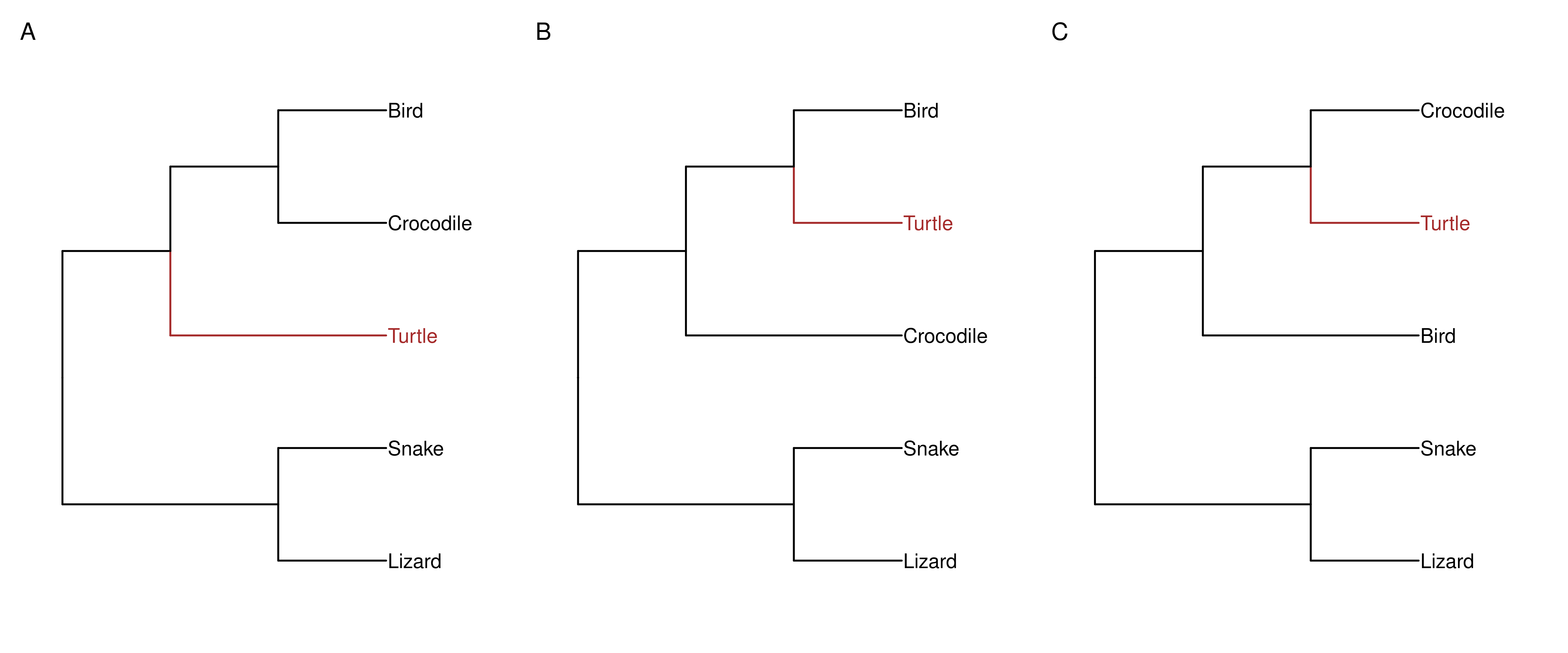
To demonstrate how to use IQ-TREE, we will use an example data set to explore a question that used to be hotly debated years ago:
Are turtles more closely-related to birds or to crocodiles?
There are 3 hypotheses to test, and here we will use maximum-likelihood-based methods to find out which one is true:
In this lesson, you will learn to:
- Infer a maximum likelihood tree
- Apply partition models and choose the best partitioning schemes
- Perform tree topology tests
- Identify and remove influential genes
- Calculate concordance factors
4.2 Data description
The data we will use in this lesson were obtained from Chiari et al. (2012), and they are stored in the data/ directory associated with this course. The files we will use are:
turtle.fa: a multiple sequence alignment (in FASTA) of a subset of the genes used in the original publication.turtle.nex: a partition file (in NEXUS) defining a subset of 29 genes.
4.3 Inferring a maximum likelihood tree
To run IQ-TREE, use the command below:
iqtree2 -s data/turtle.fa -B 1000 -T 2
Understanding the command-line arguments
The argument -s is mandatory, and this is where you indicate where the file containing the MSA is. In our previous command, iqtree2 -s data/turtle.fa means “run IQ-TREE using the MSA in the file data/turtle.fa”.
The other arguments and their meanings are:
-B: number of replicates for the ultrafast bootstrap (see Minh, Nguyen, and Von Haeseler (2013) for details). Here, we used 1000 replicates.-T: number of CPU cores to use. Here, we’re using 2 cores, because IQ-TREE defaults to using all available cores.
For a complete list of arguments and the possible values they take, run iqtree2 -h.
The main IQ-TREE report will be stored in a file ending in .iqtree, and the maximum likelihood tree (in Newick format) will be stored in a file ending in .treefile.
Exercises
Look at the report file in
data/turtle.fa.iqtreeand answer the questions below. Hint: you can use thereadLines()function to read the output to the R session.- What is the best-fit model name?
- What are the AIC/AICc/BIC scores of this model and tree?
Visualise the tree in
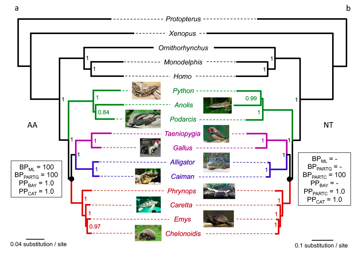
data/turtle.fa.treefile. What relationship among three trees does this tree support? What is the ultrafast bootstrap support (%) for the relevant clade?In the figure below, you can see the tree published by Chiari et al. (2012). Does the inferred tree agree with the published tree?
Solution
# Read file
turtle_report <- readLines(here("data", "turtle.fa.iqtree"))

# Q1A: Best-fit model
turtle_report[grepl("Best-fit model", turtle_report)]
[1] "Best-fit model according to BIC: GTR+F+R3"# Q1B: AIC/AICc/BIC scores for the best model
turtle_report[grepl("^Model |^GTR\\+F\\+R3", turtle_report)][1] "Model LogL AIC w-AIC AICc w-AICc BIC w-BIC"
[2] "GTR+F+R3 -116218.179 232518.358 - 0.000395 232518.524 - 0.000398 232844.049 + 0.527"# Q2
tree <- read.tree(here("data", "turtle.fa.treefile"))
plot(tree, show.node.label = TRUE)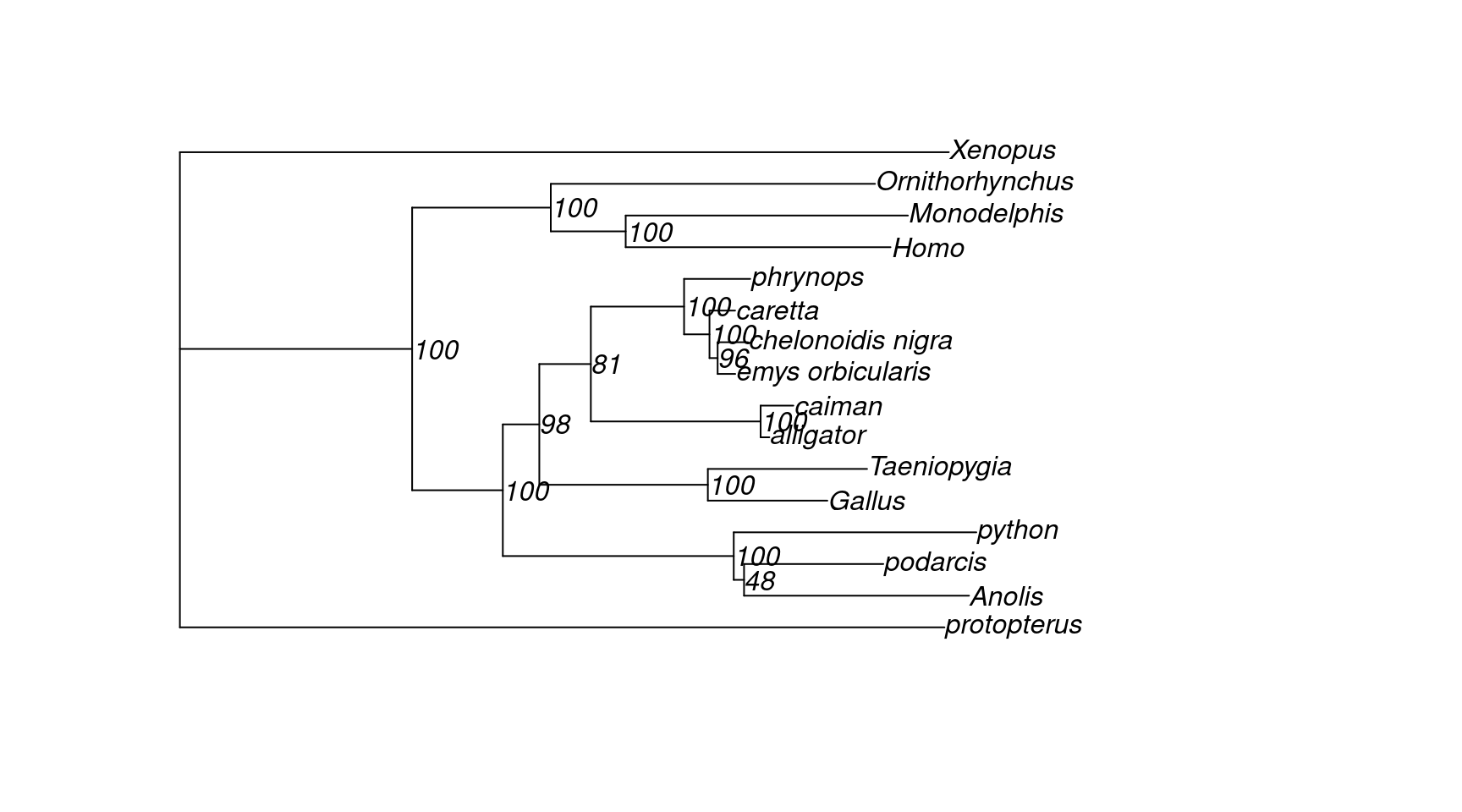
4.4 Applying partition models
Now, we will infer a ML tree applying a partition model (Chernomor, Von Haeseler, and Minh 2016), which means that each partition (specified in the turtle.nex file) will be allowed to have its own model.
iqtree2 -s data/turtle.fa -p data/turtle.nex -B 1000 -T 2
Understanding the command-line arguments
The only new argument here is -p turtle.nex, which is used to specify an edge-linked proportional partition model, so that each partition can have shorter or longer tree length (i.e., slower or faster evolutionary rates, respectively).
As in the simpler IQ-TREE run, the main report is in a file ending in .nex.iqtree, and the tree is in a file named .nex.treefile.
Exercises
Look at the report file in
data/turtle.nex.iqtree. What are the AIC/AICc/BIC scores of the partition model? Is it better than the previous model?Visualize the tree in
data/turtle.nex.treefile. What relationship among three trees does this tree support? What is the ultrafast bootstrap support (%) for the relevant clade?Does the inferred tree agree with the published tree (Chiari et al. 2012)?
Solution
# Q1
part_report <- readLines(here("data", "turtle.nex.iqtree"))
part_report[grepl("Best-fit model", part_report)]
[1] "Best-fit model according to BIC: K2P+I+G4:ENSGALG00000000223.macse_DNA_gb,K2P+G4:ENSGALG00000001529.macse_DNA_gb,TN+F+G4:ENSGALG00000002002.macse_DNA_gb,TVM+F+I+G4:ENSGALG00000002514.macse_DNA_gb,TIM2e+I+G4:ENSGALG00000003337.macse_DNA_gb,TIM2+F+G4:ENSGALG00000003700.macse_DNA_gb,TN+F+G4:ENSGALG00000003702.macse_DNA_gb,K2P+I+G4:ENSGALG00000003907.macse_DNA_gb,TNe+I:ENSGALG00000005820.macse_DNA_gb,TIM2+F+G4:ENSGALG00000005834.macse_DNA_gb,TNe+G4:ENSGALG00000005902.macse_DNA_gb,TIM3e+G4:ENSGALG00000008338.macse_DNA_gb,TPM2+F+G4:ENSGALG00000008517.macse_DNA_gb,TPM2+F+I+G4:ENSGALG00000008916.macse_DNA_gb,TIM2+F+R3:ENSGALG00000009085.macse_DNA_gb,TN+F+G4:ENSGALG00000009879.macse_DNA_gb,TPM3+F+G4:ENSGALG00000011323.macse_DNA_gb,TIM3e+I+G4:ENSGALG00000011434.macse_DNA_gb,TIM3+F+G4:ENSGALG00000011917.macse_DNA_gb,K2P+G4:ENSGALG00000011966.macse_DNA_gb,SYM+G4:ENSGALG00000012244.macse_DNA_gb,TN+F+G4:ENSGALG00000012379.macse_DNA_gb,TNe+G4:ENSGALG00000012568.macse_DNA_gb,TPM2+F+G4:ENSGALG00000013227.macse_DNA_gb,TN+F+G4:ENSGALG00000014038.macse_DNA_gb,TN+F+G4:ENSGALG00000014648.macse_DNA_gb,TIM+F+G4:ENSGALG00000015326.macse_DNA_gb,TIM2+F+G4:ENSGALG00000015397.macse_DNA_gb,TPM2+F+I+G4:ENSGALG00000016241.macse_DNA_gb"idx <- grep("List of best-fit models", part_report)
idx <- seq(idx, idx + 30)
part_report[idx] [1] "List of best-fit models per partition:"
[2] ""
[3] " ID Model LogL AIC w-AIC AICc w-AICc BIC w-BIC"
[4] " 1 K2P+I+G4 -5095.247 10198.494 + 1.42e-316 10198.541 + 5.45e-317 10217.456 + 1.24e-316"
[5] " 2 K2P+G4 -3419.486 6844.972 + 1.42e-316 6845.018 + 5.45e-317 6857.745 + 1.24e-316"
[6] " 3 TN+F+G4 -3609.176 7232.351 + 1.42e-316 7232.520 + 5.45e-317 7263.923 + 1.24e-316"
[7] " 4 TVM+F+I+G4 -4289.021 8598.043 + 1.42e-316 8598.348 + 5.45e-317 8644.001 + 1.24e-316"
[8] " 5 TIM2e+I+G4 -6224.713 12461.426 + 1.42e-316 12461.514 + 5.45e-317 12490.665 + 1.24e-316"
[9] " 6 TIM2+F+G4 -4719.062 9454.125 + 1.42e-316 9454.289 + 5.45e-317 9492.409 + 1.24e-316"
[10] " 7 TN+F+G4 -7633.586 15281.172 + 1.42e-316 15281.244 + 5.45e-317 15318.571 + 1.24e-316"
[11] " 8 K2P+I+G4 -2959.348 5926.696 + 1.42e-316 5926.780 + 5.45e-317 5943.391 + 1.24e-316"
[12] " 9 TNe+I -3109.902 6227.805 + 1.42e-316 6227.875 + 5.45e-317 6245.229 + 1.24e-316"
[13] " 10 TIM2+F+G4 -3040.697 6097.394 + 1.42e-316 6097.604 + 5.45e-317 6133.757 + 1.24e-316"
[14] " 11 TNe+G4 -2864.568 5737.135 + 1.42e-316 5737.206 + 5.45e-317 5754.518 + 1.24e-316"
[15] " 12 TIM3e+G4 -5169.589 10349.179 + 1.42e-316 10349.255 + 5.45e-317 10372.552 + 1.24e-316"
[16] " 13 TPM2+F+G4 -2702.092 5418.183 + 1.42e-316 5418.394 + 5.45e-317 5448.224 + 1.24e-316"
[17] " 14 TPM2+F+I+G4 -3667.885 7351.771 + 1.42e-316 7352.039 + 5.45e-317 7386.192 + 1.24e-316"
[18] " 15 TIM2+F+R3 -4532.069 9086.138 + 1.42e-316 9086.426 + 5.45e-317 9139.325 + 1.24e-316"
[19] " 16 TN+F+G4 -4173.396 8360.792 + 1.42e-316 8360.982 + 5.45e-317 8391.535 + 1.24e-316"
[20] " 17 TPM3+F+G4 -5262.146 10538.293 + 1.42e-316 10538.418 + 5.45e-317 10571.909 + 1.24e-316"
[21] " 18 TIM3e+I+G4 -3036.049 6084.098 + 1.42e-316 6084.289 + 5.45e-317 6108.713 + 1.24e-316"
[22] " 19 TIM3+F+G4 -4092.671 8201.341 + 1.42e-316 8201.490 + 5.45e-317 8240.450 + 1.24e-316"
[23] " 20 K2P+G4 -2968.726 5943.452 + 1.42e-316 5943.504 + 5.45e-317 5955.897 + 1.24e-316"
[24] " 21 SYM+G4 -4372.436 8758.871 + 1.42e-316 8759.022 + 5.45e-317 8791.240 + 1.24e-316"
[25] " 22 TN+F+G4 -2870.272 5754.543 + 1.42e-316 5754.763 + 5.45e-317 5784.307 + 1.24e-316"
[26] " 23 TNe+G4 -2919.575 5847.149 + 1.42e-316 5847.213 + 5.45e-317 5864.932 + 1.24e-316"
[27] " 24 TPM2+F+G4 -5568.175 11150.350 + 1.42e-316 11150.437 + 5.45e-317 11186.552 + 1.24e-316"
[28] " 25 TN+F+G4 -3315.859 6645.717 + 1.42e-316 6645.920 + 5.45e-317 6676.025 + 1.24e-316"
[29] " 26 TN+F+G4 -2097.847 4209.693 + 1.42e-316 4209.922 + 5.45e-317 4239.168 + 1.24e-316"
[30] " 27 TIM+F+G4 -3743.957 7503.913 + 1.42e-316 7504.158 + 5.45e-317 7539.049 + 1.24e-316"
[31] " 28 TIM2+F+G4 -3634.194 7284.388 + 1.42e-316 7284.634 + 5.45e-317 7319.483 + 1.24e-316"# Q2
tree <- read.tree(here("data", "turtle.nex.treefile"))
plot(tree, show.node.label = TRUE)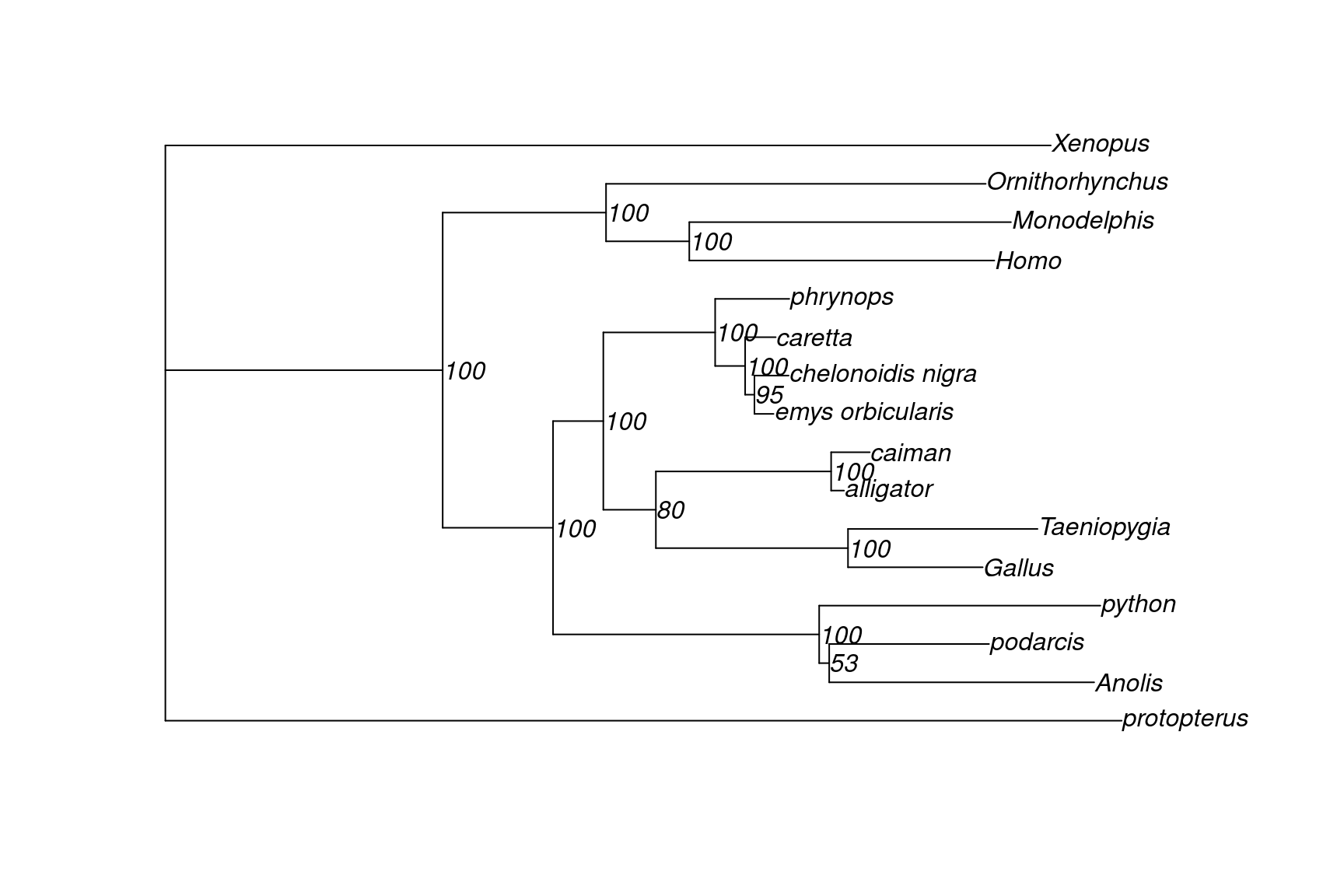
4.5 Selecting the best partitioning scheme with PartitionFinder
Now, we will use PartitionFinder (Lanfear et al. 2012) to merge partitions and reduce the potential over-parameterization.
iqtree2 -s data/turtle.fa -p data/turtle.nex -B 1000 -T 2 -m MFP+MERGE -rcluster 10 --prefix data/turtle.merge
Understanding the command-line arguments
Besides the arguments we’ve already seen, the new arguments and their meanings are:
-m: specifies the model to use. Here,MFP+MERGEindicates running PartitionFinder followed by tree reconstruction.-rcluster: to reduce computations by only examining the top n% (here, 10%) partitioning schemes using the relaxed clustering algorithm (Lanfear et al. 2014).--prefix: specifies the prefix for all output files to avoid overwriting the output of previous runs.
The main report is a file ending in .merge.iqtree, and the tree is in a file ending in .merge.treefile.
Exercises
Look at the report file
data/turtle.merge.iqtreeand answer the questions:- How many partitions do we have now?
- Look at the AIC/AICc/BIC scores. Compared with two previous models, is this model better or worse?
Visualize the tree in
data/turtle.merge.treefile. What relationship among three trees does this tree support? What is the ultrafast bootstrap support (%) for the relevant clade?Does this tree agree with the published tree (Chiari et al. 2012)?
Solution
# Read report
merge_report <- readLines(here("data", "turtle.merge.iqtree"))

# Q1A: number of partitions
merge_report[grepl("Input data:", merge_report)]
[1] "Input data: 16 taxa with 7 partitions and 20820 total sites (2.55764% missing data)"# Q1B: compare AIC/AICc/BIC scores
idx <- grep("List of best-fit models per partition", merge_report)
idx <- seq(idx, idx + 10)
merge_report[idx] [1] "List of best-fit models per partition:"
[2] ""
[3] " ID Model LogL AIC w-AIC AICc w-AICc BIC w-BIC"
[4] " 1 TPM3+F+I+G4 -33463.275 66942.550 + 3.38e-316 66942.577 + 5.45e-317 66995.241 + 2.19e-316"
[5] " 2 TIM3+F+I+G4 -28588.305 57194.610 + 3.38e-316 57194.643 + 5.45e-317 57254.076 + 2.19e-316"
[6] " 3 GTR+F+I+G4 -19434.040 38890.081 + 3.38e-316 38890.158 + 5.45e-317 38957.582 + 2.19e-316"
[7] " 4 TIM2e+I+G4 -6224.893 12461.787 + 3.38e-316 12461.874 + 5.45e-317 12491.026 + 2.19e-316"
[8] " 5 TIM2+F+G4 -17553.560 35123.120 + 3.38e-316 35123.156 + 5.45e-317 35173.507 + 2.19e-316"
[9] " 6 TVMe+I+G4 -6727.848 13469.695 + 3.38e-316 13469.809 + 5.45e-317 13504.000 + 2.19e-316"
[10] " 7 TIM+F+G4 -3743.955 7503.910 + 3.38e-316 7504.155 + 5.45e-317 7539.045 + 2.19e-316"
[11] "" # Q2
tree <- read.tree(here("data", "turtle.merge.treefile"))
plot(tree, show.node.label = TRUE)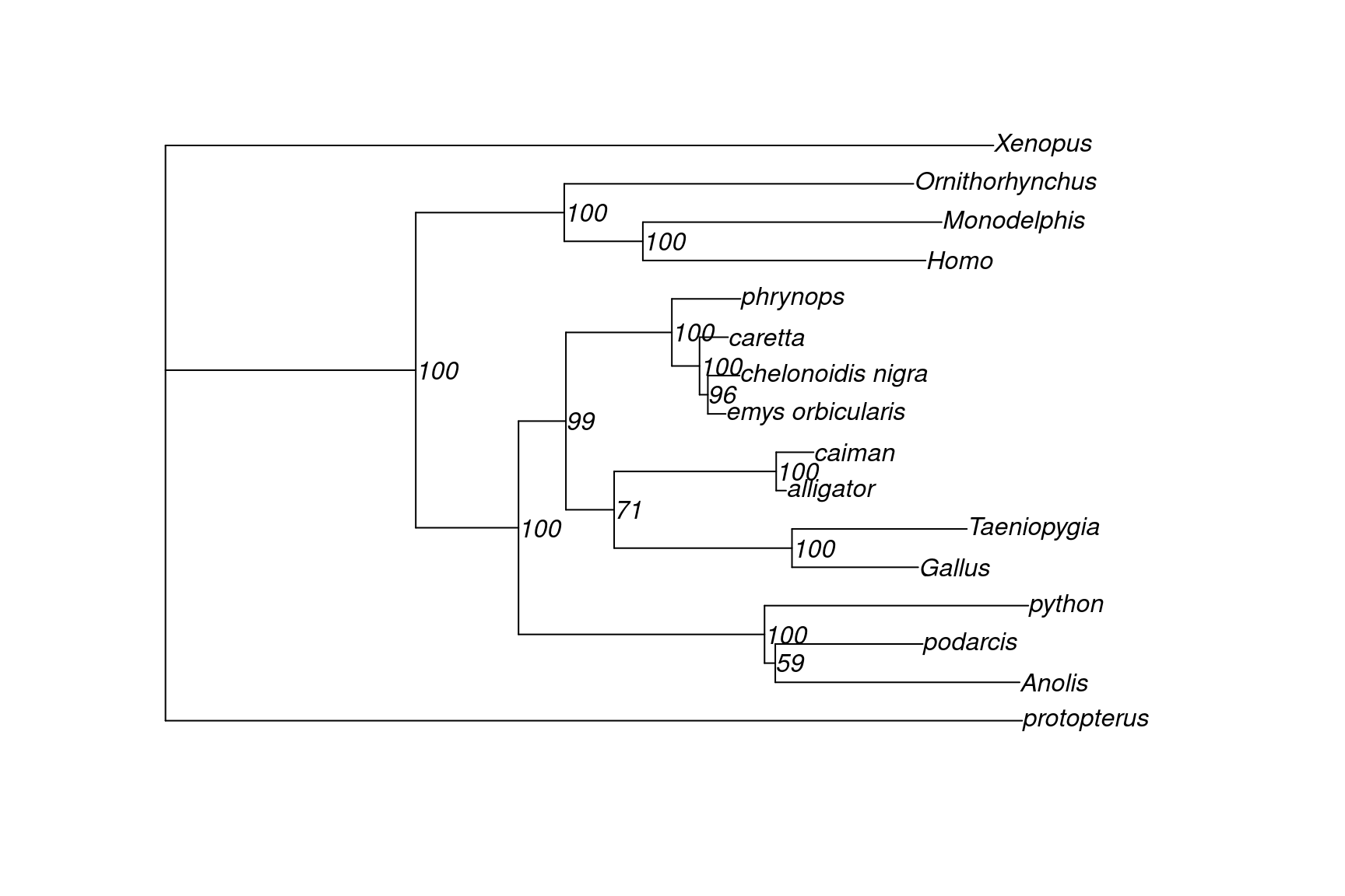
4.6 Tree topology tests
Tree topology tests can be used to find out if different trees have significant differences in log-likelihoods. To do that, you can use the SH test (Shimodaira and Hasegawa 1999) or expected likelihood weights (Strimmer and Rambaut 2002).
Before running the tests, we first need to concatenate the trees in a single file:
# Read tree inferred with a single model as plain text
tree_single <- readLines(here("data", "turtle.fa.treefile"))

# Read tree inferred with partition models as plain text
tree_partitioned <- readLines(here("data", "turtle.nex.treefile"))

# Combine trees and export to file
tree_combined <- c(tree_single, tree_partitioned)
writeLines(tree_combined, con = here("data", "turtle.trees"))
Now, we can pass the concatenated tree to IQ-TREE:
iqtree2 -s data/turtle.fa -p data/turtle.merge.best_scheme.nex \
    -z data/turtle.trees \
    -zb 10000 -au -n 0 \
    --prefix data/turtle.test
Understanding the command-line arguments
Besides the arguments we’ve already seen, the new arguments and their meanings are:
-z: path to the file containing the concatenated trees.-zb: number of replicates for approximate bootstrap for the tree topology tests (here, 10000).-au: perform the Approximately Unbiased test.-n 0: avoid tree search and just perform tree topology tests.
The main report is a file ending in .test.iqtree, and the tree is in a file ending in .test.treefile.
The KH, SH and AU tests return p-values. Thus, a tree is rejected if its p-value <0.05 (marked with a - sign).
Exercises
Look at the “USER TREES” section in the report file
data/turtle.test.iqtreeand answer the questions:- Which tree has the worst log-likelihood?
- Can you reject this tree according to the Shimodaira Hasegawa test, assuming a p-value cutoff of 0.05?
- Can you reject this tree according to the Approximately Unbiased test, assuming a p-value cutoff of 0.05?
4.7 Concordance factors
In previous analyses, we were assuming that gene trees and species tree are the same. However, in empirical data, gene trees are often different from species trees, which we call discordance. Now, we will infer different gene trees for each partition separately, and then quantify the concordance between gene trees and species tree with concordance factors.
First, let’s infer one gene tree for each partition.
iqtree2 -s data/turtle.fa -S data/turtle.nex --prefix data/turtle.loci -T 2Now, we can calculate concordance factors using the list of trees in file turtle.loci.treefile.
iqtree2 -t data/turtle.nex.treefile \
    --gcf data/turtle.loci.treefile \
    -s data/turtle.fa \
    --scf 100
The code above calculates two kinds of concordance factors:
- Gene concordance factor (gCF): percentage of decisive gene trees concordant with a particular branch of the species tree (0% <= gCF(b) <= 100%).
- Site concordance factor (sCF): percentage of decisive alignment sites supporting a particular branch of the species tree (~33% <= sCF(b) <= 100%). sCF <33% means that another discordant branch b’ is more supported, whereas sCF=100% means that branch b is supported by all sites.
Exercises
Visualize the tree in
data/turtle.nex.treefile.cf.tree. How do gCF and sCF look compared with bootstrap support values?Challenge: read concordance factors stats in file
data/turtle.nex.treefile.cf.statand create a scatterplot using {ggplot2} showing gCF in the x-axis, sCF in the y-axis, and points colored by bootstrap support values. What do you conclude?
Solution
# Q1
tree <- read.tree(here("data", "turtle.nex.treefile.cf.tree"))
plot(tree, show.node.label = TRUE)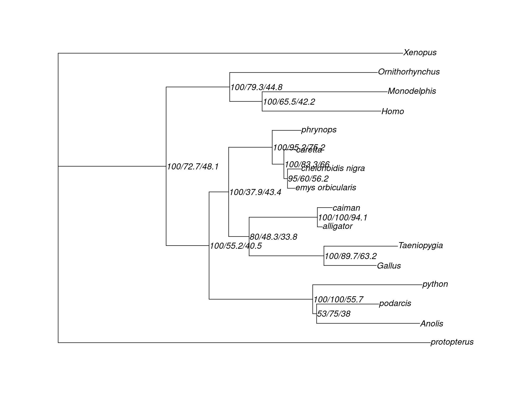
# Q2
cf_stats <- read.table(
    here("data", "turtle.nex.treefile.cf.stat"), header = TRUE
)

# Q2
library(ggplot2)
ggplot(cf_stats, aes(x = gCF, y = sCF, color = Label)) +
    geom_point(size = 3) +
    scale_color_viridis_c(direction = -1) +
    xlim(0, 100) +
    ylim(0, 100) +
    geom_abline(slope = 1, intercept = 0, linetype = "dashed")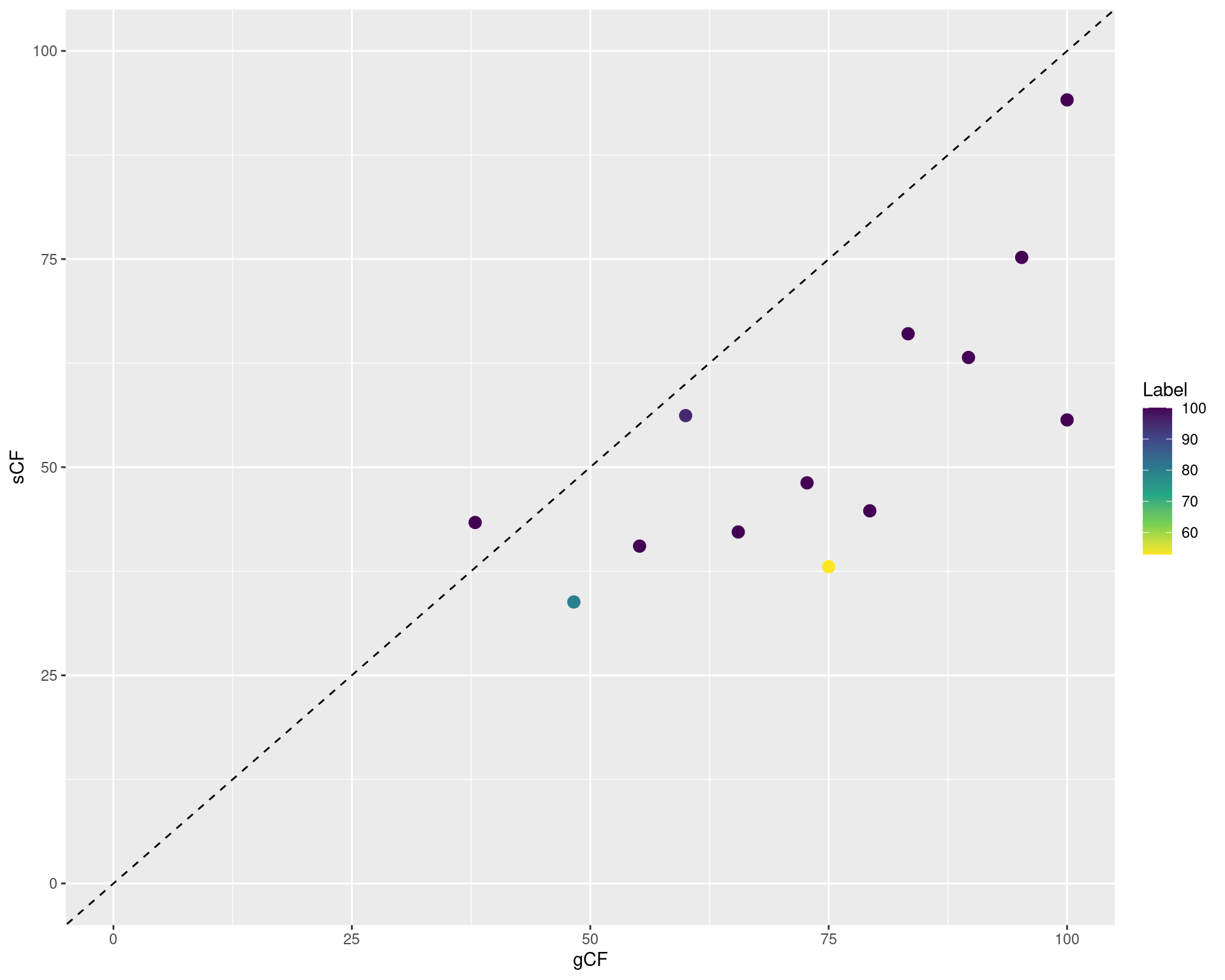
References
Chernomor, Olga, Arndt Von Haeseler, and Bui Quang Minh. 2016. “Terrace Aware Data Structure for Phylogenomic Inference from Supermatrices.” Systematic Biology 65 (6): 997–1008.
Chiari, Ylenia, Vincent Cahais, Nicolas Galtier, and Frédéric Delsuc. 2012. “Phylogenomic Analyses Support the Position of Turtles as the Sister Group of Birds and Crocodiles (Archosauria).” Bmc Biology 10: 1–15.
Lanfear, Robert, Brett Calcott, Simon YW Ho, and Stephane Guindon. 2012. “PartitionFinder: Combined Selection of Partitioning Schemes and Substitution Models for Phylogenetic Analyses.” Molecular Biology and Evolution 29 (6): 1695–1701.
Lanfear, Robert, Brett Calcott, David Kainer, Christoph Mayer, and Alexandros Stamatakis. 2014. “Selecting Optimal Partitioning Schemes for Phylogenomic Datasets.” BMC Evolutionary Biology 14: 1–14.
Minh, Bui Quang, Minh Anh Thi Nguyen, and Arndt Von Haeseler. 2013. “Ultrafast Approximation for Phylogenetic Bootstrap.” Molecular Biology and Evolution 30 (5): 1188–95.
Minh, Bui Quang, Heiko A Schmidt, Olga Chernomor, Dominik Schrempf, Michael D Woodhams, Arndt Von Haeseler, and Robert Lanfear. 2020. “IQ-TREE 2: New Models and Efficient Methods for Phylogenetic Inference in the Genomic Era.” Molecular Biology and Evolution 37 (5): 1530–34.
Shimodaira, Hidetoshi, and Masami Hasegawa. 1999. “Multiple Comparisons of Log-Likelihoods with Applications to Phylogenetic Inference.” Molecular Biology and Evolution 16 (8): 1114.
Strimmer, Korbinian, and Andrew Rambaut. 2002. “Inferring Confidence Sets of Possibly Misspecified Gene Trees.” Proceedings of the Royal Society of London. Series B: Biological Sciences 269 (1487): 137–42.