2 Data processing with the `tidyverse`

The tidyverse package is an “umbrella-package” that installs several useful packages for data analysis which work well together, such as tidyr, dplyr, ggplot2, tibble, etc. These packages help us to work and interact with the data. They allow us to do many things with your data, such as subsetting, transforming, visualizing, etc.

Let’s start by loading the tidyverse package:

library(tidyverse)
library(here)

2.1 Goals of this lesson

At the end of this lesson, you will be able to:

read tabular data from .csv/.tsv/.txt/ files
filter your data set to select particular rows and columns
add columns
summarize data
combine different data frames
reshape data from long to wide, and back

2.2 The `readr` package: reading files

The data we will use in this lesson are stored in data/rnaseq.csv. This is a comma-separated file, which means it contains a table in which columns are separated by commas. To read .csv files, we will use the function read_csv() from the readr package.

# Read csv file
rna <- read_csv(here("data", "rnaseq.csv"))

# Inspect the data
head(rna)

# A tibble: 6 × 19
  gene    sample   expression organism   age sex   infection strain  time tissue
  <chr>   <chr>         <dbl> <chr>    <dbl> <chr> <chr>     <chr>  <dbl> <chr> 
1 Asl     GSM2545…       1170 Mus mus…     8 Fema… Influenz… C57BL…     8 Cereb…
2 Apod    GSM2545…      36194 Mus mus…     8 Fema… Influenz… C57BL…     8 Cereb…
3 Cyp2d22 GSM2545…       4060 Mus mus…     8 Fema… Influenz… C57BL…     8 Cereb…
4 Klk6    GSM2545…        287 Mus mus…     8 Fema… Influenz… C57BL…     8 Cereb…
5 Fcrls   GSM2545…         85 Mus mus…     8 Fema… Influenz… C57BL…     8 Cereb…
6 Slc2a4  GSM2545…        782 Mus mus…     8 Fema… Influenz… C57BL…     8 Cereb…
# ℹ 9 more variables: mouse <dbl>, ENTREZID <dbl>, product <chr>,
#   ensembl_gene_id <chr>, external_synonym <chr>, chromosome_name <chr>,
#   gene_biotype <chr>, phenotype_description <chr>,
#   hsapiens_homolog_associated_gene_name <chr>

Notice that the class of the data is now referred to as a tibble.

Tibbles tweak some of the behaviors of the data frame objects we introduced in the previously. The data structure is very similar to a data frame. For our purposes the only differences are that:

It displays the data type of each column under its name. Note that <dbl> is a data type defined to hold numeric values with decimal points.
It only prints the first few rows of data and only as many columns as fit on one screen.

2.3 The `dplyr` package: filtering, extending, and summarizing data

The dplyr is one of the most main packages of the tidyverse, and it can be used to perform all sorts of day-to-day data processing. Here, we are going to learn some of the most common dplyr functions:

select(): subset columns
filter(): subset rows on conditions
mutate(): create new columns by using information from other columns
group_by() and summarise(): create summary statistics on grouped data
arrange(): sort results
count(): count discrete values

2.3.1 Selecting columns and filtering rows

To select columns of a data frame, use select(). The first argument to this function is the data frame (rna), and the subsequent arguments are the columns to keep.

select(rna, gene, sample, tissue, expression)

# A tibble: 32,428 × 4
   gene    sample     tissue     expression
   <chr>   <chr>      <chr>           <dbl>
 1 Asl     GSM2545336 Cerebellum       1170
 2 Apod    GSM2545336 Cerebellum      36194
 3 Cyp2d22 GSM2545336 Cerebellum       4060
 4 Klk6    GSM2545336 Cerebellum        287
 5 Fcrls   GSM2545336 Cerebellum         85
 6 Slc2a4  GSM2545336 Cerebellum        782
 7 Exd2    GSM2545336 Cerebellum       1619
 8 Gjc2    GSM2545336 Cerebellum        288
 9 Plp1    GSM2545336 Cerebellum      43217
10 Gnb4    GSM2545336 Cerebellum       1071
# ℹ 32,418 more rows

To select all columns except certain ones, put a “-” in front of the variable to exclude it. For example, to select all columns but tissue and organism, you’d use:

select(rna, -tissue, -organism)

# A tibble: 32,428 × 17
   gene    sample   expression   age sex   infection strain  time mouse ENTREZID
   <chr>   <chr>         <dbl> <dbl> <chr> <chr>     <chr>  <dbl> <dbl>    <dbl>
 1 Asl     GSM2545…       1170     8 Fema… Influenz… C57BL…     8    14   109900
 2 Apod    GSM2545…      36194     8 Fema… Influenz… C57BL…     8    14    11815
 3 Cyp2d22 GSM2545…       4060     8 Fema… Influenz… C57BL…     8    14    56448
 4 Klk6    GSM2545…        287     8 Fema… Influenz… C57BL…     8    14    19144
 5 Fcrls   GSM2545…         85     8 Fema… Influenz… C57BL…     8    14    80891
 6 Slc2a4  GSM2545…        782     8 Fema… Influenz… C57BL…     8    14    20528
 7 Exd2    GSM2545…       1619     8 Fema… Influenz… C57BL…     8    14    97827
 8 Gjc2    GSM2545…        288     8 Fema… Influenz… C57BL…     8    14   118454
 9 Plp1    GSM2545…      43217     8 Fema… Influenz… C57BL…     8    14    18823
10 Gnb4    GSM2545…       1071     8 Fema… Influenz… C57BL…     8    14    14696
# ℹ 32,418 more rows
# ℹ 7 more variables: product <chr>, ensembl_gene_id <chr>,
#   external_synonym <chr>, chromosome_name <chr>, gene_biotype <chr>,
#   phenotype_description <chr>, hsapiens_homolog_associated_gene_name <chr>

To choose rows based on specific criteria, use filter():

filter(rna, sex == "Male")

# A tibble: 14,740 × 19
   gene    sample  expression organism   age sex   infection strain  time tissue
   <chr>   <chr>        <dbl> <chr>    <dbl> <chr> <chr>     <chr>  <dbl> <chr> 
 1 Asl     GSM254…        626 Mus mus…     8 Male  Influenz… C57BL…     4 Cereb…
 2 Apod    GSM254…      13021 Mus mus…     8 Male  Influenz… C57BL…     4 Cereb…
 3 Cyp2d22 GSM254…       2171 Mus mus…     8 Male  Influenz… C57BL…     4 Cereb…
 4 Klk6    GSM254…        448 Mus mus…     8 Male  Influenz… C57BL…     4 Cereb…
 5 Fcrls   GSM254…        180 Mus mus…     8 Male  Influenz… C57BL…     4 Cereb…
 6 Slc2a4  GSM254…        313 Mus mus…     8 Male  Influenz… C57BL…     4 Cereb…
 7 Exd2    GSM254…       2366 Mus mus…     8 Male  Influenz… C57BL…     4 Cereb…
 8 Gjc2    GSM254…        310 Mus mus…     8 Male  Influenz… C57BL…     4 Cereb…
 9 Plp1    GSM254…      53126 Mus mus…     8 Male  Influenz… C57BL…     4 Cereb…
10 Gnb4    GSM254…       1355 Mus mus…     8 Male  Influenz… C57BL…     4 Cereb…
# ℹ 14,730 more rows
# ℹ 9 more variables: mouse <dbl>, ENTREZID <dbl>, product <chr>,
#   ensembl_gene_id <chr>, external_synonym <chr>, chromosome_name <chr>,
#   gene_biotype <chr>, phenotype_description <chr>,
#   hsapiens_homolog_associated_gene_name <chr>

filter(rna, sex == "Male" & infection == "NonInfected")

# A tibble: 4,422 × 19
   gene    sample  expression organism   age sex   infection strain  time tissue
   <chr>   <chr>        <dbl> <chr>    <dbl> <chr> <chr>     <chr>  <dbl> <chr> 
 1 Asl     GSM254…        535 Mus mus…     8 Male  NonInfec… C57BL…     0 Cereb…
 2 Apod    GSM254…      13668 Mus mus…     8 Male  NonInfec… C57BL…     0 Cereb…
 3 Cyp2d22 GSM254…       2008 Mus mus…     8 Male  NonInfec… C57BL…     0 Cereb…
 4 Klk6    GSM254…       1101 Mus mus…     8 Male  NonInfec… C57BL…     0 Cereb…
 5 Fcrls   GSM254…        375 Mus mus…     8 Male  NonInfec… C57BL…     0 Cereb…
 6 Slc2a4  GSM254…        249 Mus mus…     8 Male  NonInfec… C57BL…     0 Cereb…
 7 Exd2    GSM254…       3126 Mus mus…     8 Male  NonInfec… C57BL…     0 Cereb…
 8 Gjc2    GSM254…        791 Mus mus…     8 Male  NonInfec… C57BL…     0 Cereb…
 9 Plp1    GSM254…      98658 Mus mus…     8 Male  NonInfec… C57BL…     0 Cereb…
10 Gnb4    GSM254…       2437 Mus mus…     8 Male  NonInfec… C57BL…     0 Cereb…
# ℹ 4,412 more rows
# ℹ 9 more variables: mouse <dbl>, ENTREZID <dbl>, product <chr>,
#   ensembl_gene_id <chr>, external_synonym <chr>, chromosome_name <chr>,
#   gene_biotype <chr>, phenotype_description <chr>,
#   hsapiens_homolog_associated_gene_name <chr>

Now, let’s imagine we are interested in the human homologs of the mouse genes analyzed in this dataset. This information can be found in the last column of the rna tibble, named hsapiens_homolog_associated_gene_name. To visualise it easily, we will create a new table containing just the 2 columns gene and hsapiens_homolog_associated_gene_name.

genes <- select(rna, gene, hsapiens_homolog_associated_gene_name)
genes

# A tibble: 32,428 × 2
   gene    hsapiens_homolog_associated_gene_name
   <chr>   <chr>                                
 1 Asl     ASL                                  
 2 Apod    APOD                                 
 3 Cyp2d22 CYP2D6                               
 4 Klk6    KLK6                                 
 5 Fcrls   FCRL2                                
 6 Slc2a4  SLC2A4                               
 7 Exd2    EXD2                                 
 8 Gjc2    GJC2                                 
 9 Plp1    PLP1                                 
10 Gnb4    GNB4                                 
# ℹ 32,418 more rows

A very nice thing about tidyverse verbs (functions) is that they can be executed one after the other by using the pipe operator (|> or %>%). In practice, that means you don’t have to create intermediate objects for complicated subsetting operations that involve multiple steps. The pipe operator is often read as and then in the sense that you apply a function A and then you pass the output to function B, and then you pass the output to function C, and so on and so forth. For example:

1rna |>
2    filter(sex == "Male") |>
3    select(gene, sample, tissue, expression)

1: Take the object rna, and then
2: filter it to keep only rows that have “Male” in the column sex, and then
3: select the columns gene, sample, tissue, expression

# A tibble: 14,740 × 4
   gene    sample     tissue     expression
   <chr>   <chr>      <chr>           <dbl>
 1 Asl     GSM2545340 Cerebellum        626
 2 Apod    GSM2545340 Cerebellum      13021
 3 Cyp2d22 GSM2545340 Cerebellum       2171
 4 Klk6    GSM2545340 Cerebellum        448
 5 Fcrls   GSM2545340 Cerebellum        180
 6 Slc2a4  GSM2545340 Cerebellum        313
 7 Exd2    GSM2545340 Cerebellum       2366
 8 Gjc2    GSM2545340 Cerebellum        310
 9 Plp1    GSM2545340 Cerebellum      53126
10 Gnb4    GSM2545340 Cerebellum       1355
# ℹ 14,730 more rows

Practice

Using pipes, subset the rna tibble to keep observations that match the following criteria:

Female mice
Time point 0
Expression higher than 50000

Then, select the columns gene, sample, time, expression, and age.

Filter rna to keep observations for infected samples, then count the number of rows. Hint: use the unique() function to see all the unique observations in a column, and the nrow() function the get the number of rows in a data frame/tibble.
Do the same as above, but now keep only non-infected samples.

Show me the solutions

# Q1
rna |>
  filter(
      sex == "Female",
      time == 0,
      expression > 50000
  ) |>
  select(gene, sample, time, expression, age)

# A tibble: 9 × 5
  gene   sample      time expression   age
  <chr>  <chr>      <dbl>      <dbl> <dbl>
1 Plp1   GSM2545337     0     101241     8
2 Atp1b1 GSM2545337     0      53260     8
3 Plp1   GSM2545338     0      96534     8
4 Atp1b1 GSM2545338     0      50614     8
5 Plp1   GSM2545348     0     102790     8
6 Atp1b1 GSM2545348     0      59544     8
7 Plp1   GSM2545353     0      71237     8
8 Glul   GSM2545353     0      52451     8
9 Atp1b1 GSM2545353     0      61451     8

# Q2
rna |> 
    filter(infection == "InfluenzaA") |>
    nrow()

[1] 22110

# Q3
rna |>
    filter(infection == "NonInfected") |>
    nrow()

[1] 10318

2.3.2 Adding new columns

Frequently you’ll want to create new columns based on the values of existing columns, for example to do unit conversions, or to find the ratio of values in two columns. For this, we’ll use mutate().

For example, the column time contains the time in days. Let’s create a new column named time_hours that contains the time in hours.

rna |>
    mutate(time_hours = time * 24) |>
    select(time, time_hours)

# A tibble: 32,428 × 2
    time time_hours
   <dbl>      <dbl>
 1     8        192
 2     8        192
 3     8        192
 4     8        192
 5     8        192
 6     8        192
 7     8        192
 8     8        192
 9     8        192
10     8        192
# ℹ 32,418 more rows

You can also create a second new column based on the first new column within the same call of mutate():

rna |>
    mutate(
        time_hours = time * 24,
        time_minutes = time_hours * 60
    ) |>
    select(time, time_hours, time_minutes)

# A tibble: 32,428 × 3
    time time_hours time_minutes
   <dbl>      <dbl>        <dbl>
 1     8        192        11520
 2     8        192        11520
 3     8        192        11520
 4     8        192        11520
 5     8        192        11520
 6     8        192        11520
 7     8        192        11520
 8     8        192        11520
 9     8        192        11520
10     8        192        11520
# ℹ 32,418 more rows

Practice

Create a new data frame from the rna data that meets the following criteria: contains only the gene, chromosome_name, phenotype_description, sample, and expression columns. The expression values should be log-transformed. This data frame must only contain genes located on sex chromosomes, associated with a phenotype_description, and with a log expression higher than 5.

Hint: think about how the commands should be ordered to produce this data frame!

Show me the solutions

rna |>
  mutate(expression = log(expression)) |>
  select(gene, chromosome_name, phenotype_description, sample, expression) |>
  filter(chromosome_name == "X" | chromosome_name == "Y") |>
  filter(!is.na(phenotype_description)) |>
  filter(expression > 5)

# A tibble: 649 × 5
   gene   chromosome_name phenotype_description                sample expression
   <chr>  <chr>           <chr>                                <chr>       <dbl>
 1 Plp1   X               abnormal CNS glial cell morphology   GSM25…      10.7 
 2 Slc7a3 X               decreased body length                GSM25…       5.46
 3 Plxnb3 X               abnormal coat appearance             GSM25…       6.58
 4 Rbm3   X               abnormal liver morphology            GSM25…       9.32
 5 Cfp    X               abnormal cardiovascular system phys… GSM25…       6.18
 6 Ebp    X               abnormal embryonic erythrocyte morp… GSM25…       6.68
 7 Cd99l2 X               abnormal cellular extravasation      GSM25…       8.04
 8 Piga   X               abnormal brain development           GSM25…       6.06
 9 Pim2   X               decreased T cell proliferation       GSM25…       7.11
10 Itm2a  X               no abnormal phenotype detected       GSM25…       7.48
# ℹ 639 more rows

2.3.3 Summarizing grouped data

Many data analysis tasks can be approached using the split-apply-combine paradigm: split the data into groups, apply some analysis to each group, and then combine the results. dplyr makes this very easy through the use of the group_by() function.

rna %>%
  group_by(gene)

# A tibble: 32,428 × 19
# Groups:   gene [1,474]
   gene    sample  expression organism   age sex   infection strain  time tissue
   <chr>   <chr>        <dbl> <chr>    <dbl> <chr> <chr>     <chr>  <dbl> <chr> 
 1 Asl     GSM254…       1170 Mus mus…     8 Fema… Influenz… C57BL…     8 Cereb…
 2 Apod    GSM254…      36194 Mus mus…     8 Fema… Influenz… C57BL…     8 Cereb…
 3 Cyp2d22 GSM254…       4060 Mus mus…     8 Fema… Influenz… C57BL…     8 Cereb…
 4 Klk6    GSM254…        287 Mus mus…     8 Fema… Influenz… C57BL…     8 Cereb…
 5 Fcrls   GSM254…         85 Mus mus…     8 Fema… Influenz… C57BL…     8 Cereb…
 6 Slc2a4  GSM254…        782 Mus mus…     8 Fema… Influenz… C57BL…     8 Cereb…
 7 Exd2    GSM254…       1619 Mus mus…     8 Fema… Influenz… C57BL…     8 Cereb…
 8 Gjc2    GSM254…        288 Mus mus…     8 Fema… Influenz… C57BL…     8 Cereb…
 9 Plp1    GSM254…      43217 Mus mus…     8 Fema… Influenz… C57BL…     8 Cereb…
10 Gnb4    GSM254…       1071 Mus mus…     8 Fema… Influenz… C57BL…     8 Cereb…
# ℹ 32,418 more rows
# ℹ 9 more variables: mouse <dbl>, ENTREZID <dbl>, product <chr>,
#   ensembl_gene_id <chr>, external_synonym <chr>, chromosome_name <chr>,
#   gene_biotype <chr>, phenotype_description <chr>,
#   hsapiens_homolog_associated_gene_name <chr>

The group_by() function doesn’t perform any data processing, it groups the data into subsets: in the example above, our initial tibble of 32428 observations is split into 1474 groups based on the gene variable.

Once the data has been grouped, subsequent operations will be applied on each group independently by using the summarise() function. For example, to compute the mean expression by gene, you’d do:

rna |>
    group_by(gene) |>
    summarise(mean_expression = mean(expression))

# A tibble: 1,474 × 2
   gene     mean_expression
   <chr>              <dbl>
 1 AI504432         1053.  
 2 AW046200          131.  
 3 AW551984          295.  
 4 Aamp             4751.  
 5 Abca12              4.55
 6 Abcc8            2498.  
 7 Abhd14a           525.  
 8 Abi2             4909.  
 9 Abi3bp           1002.  
10 Abl2             2124.  
# ℹ 1,464 more rows

We could also calculate the mean expression levels of all genes in each sample:

rna |>
  group_by(sample) |>
  summarise(mean_expression = mean(expression))

# A tibble: 22 × 2
   sample     mean_expression
   <chr>                <dbl>
 1 GSM2545336           2062.
 2 GSM2545337           1766.
 3 GSM2545338           1668.
 4 GSM2545339           1696.
 5 GSM2545340           1682.
 6 GSM2545341           1638.
 7 GSM2545342           1594.
 8 GSM2545343           2107.
 9 GSM2545344           1712.
10 GSM2545345           1700.
# ℹ 12 more rows

But we can can also group by multiple columns:

rna |>
  group_by(gene, infection, time) |>
  summarise(mean_expression = mean(expression))

# A tibble: 4,422 × 4
# Groups:   gene, infection [2,948]
   gene     infection    time mean_expression
   <chr>    <chr>       <dbl>           <dbl>
 1 AI504432 InfluenzaA      4           1104.
 2 AI504432 InfluenzaA      8           1014 
 3 AI504432 NonInfected     0           1034.
 4 AW046200 InfluenzaA      4            152.
 5 AW046200 InfluenzaA      8             81 
 6 AW046200 NonInfected     0            155.
 7 AW551984 InfluenzaA      4            302.
 8 AW551984 InfluenzaA      8            342.
 9 AW551984 NonInfected     0            238 
10 Aamp     InfluenzaA      4           4870 
# ℹ 4,412 more rows

Practice

Calculate the mean and median expression of all genes.
Calculate the mean expression level of gene “Dok3” by timepoints.

Show me the solutions

# Q1
rna |>
    group_by(gene) |>
    summarise(
        mean_exp = mean(expression),
        median_exp = median(expression)
    )

# A tibble: 1,474 × 3
   gene     mean_exp median_exp
   <chr>       <dbl>      <dbl>
 1 AI504432  1053.        1008 
 2 AW046200   131.         130.
 3 AW551984   295.         273 
 4 Aamp      4751.        4716.
 5 Abca12       4.55         5 
 6 Abcc8     2498.        2367 
 7 Abhd14a    525.         503 
 8 Abi2      4909.        4820.
 9 Abi3bp    1002.        1008.
10 Abl2      2124.        2134.
# ℹ 1,464 more rows

# Q2
rna |>
  filter(gene == "Dok3") |>
  group_by(time) |>
  summarise(mean = mean(expression))

# A tibble: 3 × 2
   time  mean
  <dbl> <dbl>
1     0  169 
2     4  156.
3     8   61

2.3.4 Counting observations per group

When working with data, we often want to know the number of observations found for each factor or combination of factors. For this task, dplyr provides count(). For example, if we wanted to count the number of rows of data for each infected and non-infected samples, we would do:

rna |>
    count(infection)

# A tibble: 2 × 2
  infection       n
  <chr>       <int>
1 InfluenzaA  22110
2 NonInfected 10318

If we wanted to count a combination of factors, such as infection and time, we would specify the first and the second factor as the arguments of count():

rna |>
    count(infection, time)

# A tibble: 3 × 3
  infection    time     n
  <chr>       <dbl> <int>
1 InfluenzaA      4 11792
2 InfluenzaA      8 10318
3 NonInfected     0 10318

It is sometimes useful to sort the result to facilitate the comparisons. We can use arrange() to sort the table. For instance, we might want to arrange the table above by time:

# Ascending order
rna |>
  count(infection, time) |>
  arrange(time)

# A tibble: 3 × 3
  infection    time     n
  <chr>       <dbl> <int>
1 NonInfected     0 10318
2 InfluenzaA      4 11792
3 InfluenzaA      8 10318

# Descending order
rna |>
  count(infection, time) |>
  arrange(-time)

# A tibble: 3 × 3
  infection    time     n
  <chr>       <dbl> <int>
1 InfluenzaA      8 10318
2 InfluenzaA      4 11792
3 NonInfected     0 10318

Practice

How many genes were analyzed in each sample?
Use group_by() and summarise() to evaluate the sequencing depth (the sum of all counts) in each sample. Which sample has the highest sequencing depth?
Pick one sample and evaluate the number of genes by biotype.
Identify genes associated with the “abnormal DNA methylation” phenotype description, and calculate their mean expression (in log) at time 0, time 4 and time 8.

Show me the solutions

# Q1
rna |>
  count(sample)

# A tibble: 22 × 2
   sample         n
   <chr>      <int>
 1 GSM2545336  1474
 2 GSM2545337  1474
 3 GSM2545338  1474
 4 GSM2545339  1474
 5 GSM2545340  1474
 6 GSM2545341  1474
 7 GSM2545342  1474
 8 GSM2545343  1474
 9 GSM2545344  1474
10 GSM2545345  1474
# ℹ 12 more rows

# Q2
rna |>
  group_by(sample) |>
  summarise(seq_depth = sum(expression)) |>
  arrange(-seq_depth)

# A tibble: 22 × 2
   sample     seq_depth
   <chr>          <dbl>
 1 GSM2545350   3255566
 2 GSM2545352   3216163
 3 GSM2545343   3105652
 4 GSM2545336   3039671
 5 GSM2545380   3036098
 6 GSM2545353   2953249
 7 GSM2545348   2913678
 8 GSM2545362   2913517
 9 GSM2545351   2782464
10 GSM2545349   2758006
# ℹ 12 more rows

# Q3
rna |>
  filter(sample == "GSM2545336") |>
  count(gene_biotype) |>
  arrange(-n)

# A tibble: 13 × 2
   gene_biotype                           n
   <chr>                              <int>
 1 protein_coding                      1321
 2 lncRNA                                69
 3 processed_pseudogene                  59
 4 miRNA                                  7
 5 snoRNA                                 5
 6 TEC                                    4
 7 polymorphic_pseudogene                 2
 8 unprocessed_pseudogene                 2
 9 IG_C_gene                              1
10 scaRNA                                 1
11 transcribed_processed_pseudogene       1
12 transcribed_unitary_pseudogene         1
13 transcribed_unprocessed_pseudogene     1

# Q4
rna |>
  filter(phenotype_description == "abnormal DNA methylation") |>
  group_by(gene, time) |>
  summarise(mean_expression = mean(log(expression))) |>
  arrange()

# A tibble: 6 × 3
# Groups:   gene [2]
  gene   time mean_expression
  <chr> <dbl>           <dbl>
1 Xist      0            6.95
2 Xist      4            6.34
3 Xist      8            7.13
4 Zdbf2     0            6.27
5 Zdbf2     4            6.27
6 Zdbf2     8            6.19

2.3.5 Joining tables

In many real-life situations, data are spread across multiple tables. A common example in transcriptomics is to have gene expression in one table, and functional annotation for each gene in another table. In these cases, one may want to combine the two tables based on a column in common.

Joining tables can be done with the dplyr functions inner_join(), full_join(), left_join(), and right_join(), each of which are exemplified in the figure below:

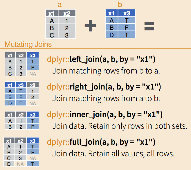
To demonstrate that, let’s first create a data frame with the mean expression of the genes Asl, Apod, and Klk6.

# Mean expression of the genes `Asl`, `Apod`, and Klk6
mean_exp <- rna |>
    filter(gene %in% c("Asl", "Apod", "Klk6")) |>
    group_by(gene) |>
    summarise(mean_exp = mean(expression))

Next, we will load a table with genes and their descriptions, available in data/gene_descriptions.csv.

# Read data
descriptions <- read_csv(here("data", "gene_descriptions.csv"))

# Inspect data
head(descriptions)

# A tibble: 6 × 2
  gene    gene_description                                                      
  <chr>   <chr>                                                                 
1 Cyp2d22 cytochrome P450, family 2, subfamily d, polypeptide 22 [Source:MGI Sy…
2 Klk6    kallikrein related-peptidase 6 [Source:MGI Symbol;Acc:MGI:1343166]    
3 Fcrls   Fc receptor-like S, scavenger receptor [Source:MGI Symbol;Acc:MGI:193…
4 Plp1    proteolipid protein (myelin) 1 [Source:MGI Symbol;Acc:MGI:97623]      
5 Exd2    exonuclease 3'-5' domain containing 2 [Source:MGI Symbol;Acc:MGI:1922…
6 Apod    apolipoprotein D [Source:MGI Symbol;Acc:MGI:88056]

Now, we will combine the two tables so that we have the mean expression for each gene + gene descriptions in a single table. To combine the two tables while keeping only genes present in the column gene of both tables, we will use the function inner_join().

inner_join(mean_exp, descriptions)

# A tibble: 3 × 3
  gene  mean_exp gene_description                                               
  <chr>    <dbl> <chr>                                                          
1 Apod    18968. apolipoprotein D [Source:MGI Symbol;Acc:MGI:88056]             
2 Asl       708. argininosuccinate lyase [Source:MGI Symbol;Acc:MGI:88084]      
3 Klk6      554. kallikrein related-peptidase 6 [Source:MGI Symbol;Acc:MGI:1343…

Challenge

Join the tables mean_exp and descriptions using the function full_join(). How does the output change?

Show me the solutions

full_join(mean_exp, descriptions)

# A tibble: 10 × 3
   gene    mean_exp gene_description                                            
   <chr>      <dbl> <chr>                                                       
 1 Apod      18968. apolipoprotein D [Source:MGI Symbol;Acc:MGI:88056]          
 2 Asl         708. argininosuccinate lyase [Source:MGI Symbol;Acc:MGI:88084]   
 3 Klk6        554. kallikrein related-peptidase 6 [Source:MGI Symbol;Acc:MGI:1…
 4 Cyp2d22      NA  cytochrome P450, family 2, subfamily d, polypeptide 22 [Sou…
 5 Fcrls        NA  Fc receptor-like S, scavenger receptor [Source:MGI Symbol;A…
 6 Plp1         NA  proteolipid protein (myelin) 1 [Source:MGI Symbol;Acc:MGI:9…
 7 Exd2         NA  exonuclease 3'-5' domain containing 2 [Source:MGI Symbol;Ac…
 8 Gnb4         NA  guanine nucleotide binding protein (G protein), beta 4 [Sou…
 9 Slc2a4       NA  solute carrier family 2 (facilitated glucose transporter), …
10 Gjc2         NA  gap junction protein, gamma 2 [Source:MGI Symbol;Acc:MGI:21…

2.4 The `tidyr` package: from long to wide, and vice versa

In the rna tibble, the rows contain expression values (the unit) that are associated with a combination of 2 other variables: gene and sample.

All the other columns correspond to variables describing either the sample (organism, age, sex, …) or the gene (gene_biotype, ENTREZ_ID, product, …). The variables that don’t change with genes or with samples will have the same value in all the rows.

rna |>
  arrange(gene)

# A tibble: 32,428 × 19
   gene     sample expression organism   age sex   infection strain  time tissue
   <chr>    <chr>       <dbl> <chr>    <dbl> <chr> <chr>     <chr>  <dbl> <chr> 
 1 AI504432 GSM25…       1230 Mus mus…     8 Fema… Influenz… C57BL…     8 Cereb…
 2 AI504432 GSM25…       1085 Mus mus…     8 Fema… NonInfec… C57BL…     0 Cereb…
 3 AI504432 GSM25…        969 Mus mus…     8 Fema… NonInfec… C57BL…     0 Cereb…
 4 AI504432 GSM25…       1284 Mus mus…     8 Fema… Influenz… C57BL…     4 Cereb…
 5 AI504432 GSM25…        966 Mus mus…     8 Male  Influenz… C57BL…     4 Cereb…
 6 AI504432 GSM25…        918 Mus mus…     8 Male  Influenz… C57BL…     8 Cereb…
 7 AI504432 GSM25…        985 Mus mus…     8 Fema… Influenz… C57BL…     8 Cereb…
 8 AI504432 GSM25…        972 Mus mus…     8 Male  NonInfec… C57BL…     0 Cereb…
 9 AI504432 GSM25…       1000 Mus mus…     8 Fema… Influenz… C57BL…     4 Cereb…
10 AI504432 GSM25…        816 Mus mus…     8 Male  Influenz… C57BL…     4 Cereb…
# ℹ 32,418 more rows
# ℹ 9 more variables: mouse <dbl>, ENTREZID <dbl>, product <chr>,
#   ensembl_gene_id <chr>, external_synonym <chr>, chromosome_name <chr>,
#   gene_biotype <chr>, phenotype_description <chr>,
#   hsapiens_homolog_associated_gene_name <chr>

This structure is called a long-format, as one column contains all the values, and other column(s) list(s) the context of the value.

In certain cases, the long-format is not really “human-readable”, and another format, a wide-format is preferred, as a more compact way of representing the data. This is typically the case with gene expression values that scientists are used to look as matrices, were rows represent genes and columns represent samples.

In this format, it would therefore become straightforward to explore the relationship between the gene expression levels within, and between, the samples.

# A tibble: 1,474 × 23
   gene    GSM2545336 GSM2545337 GSM2545338 GSM2545339 GSM2545340 GSM2545341
   <chr>        <dbl>      <dbl>      <dbl>      <dbl>      <dbl>      <dbl>
 1 Asl           1170        361        400        586        626        988
 2 Apod         36194      10347       9173      10620      13021      29594
 3 Cyp2d22       4060       1616       1603       1901       2171       3349
 4 Klk6           287        629        641        578        448        195
 5 Fcrls           85        233        244        237        180         38
 6 Slc2a4         782        231        248        265        313        786
 7 Exd2          1619       2288       2235       2513       2366       1359
 8 Gjc2           288        595        568        551        310        146
 9 Plp1         43217     101241      96534      58354      53126      27173
10 Gnb4          1071       1791       1867       1430       1355        798
# ℹ 1,464 more rows
# ℹ 16 more variables: GSM2545342 <dbl>, GSM2545343 <dbl>, GSM2545344 <dbl>,
#   GSM2545345 <dbl>, GSM2545346 <dbl>, GSM2545347 <dbl>, GSM2545348 <dbl>,
#   GSM2545349 <dbl>, GSM2545350 <dbl>, GSM2545351 <dbl>, GSM2545352 <dbl>,
#   GSM2545353 <dbl>, GSM2545354 <dbl>, GSM2545362 <dbl>, GSM2545363 <dbl>,
#   GSM2545380 <dbl>

To convert the gene expression values from rna into a wide format, we need to create a new table where the values of the sample column would become the names of column variables.

The key point here is that we are still following a tidy data structure, but we have reshaped the data according to the observations of interest: expression levels per gene instead of recording them per gene and per sample.

Reshaping data from long to wide format can be performed with the function pivot_wider() from tidyr. For example:

rna_wide <- rna |>                            
1    select(gene, sample, expression) |>
    pivot_wider(
2        names_from = sample,
3        values_from = expression
    )

rna_wide

1: Select columns gene, sample, and expression
2: Columns names of the wide table will be the values of the sample column
3: Values in the wide table will be the values of the expression column

# A tibble: 1,474 × 23
   gene    GSM2545336 GSM2545337 GSM2545338 GSM2545339 GSM2545340 GSM2545341
   <chr>        <dbl>      <dbl>      <dbl>      <dbl>      <dbl>      <dbl>
 1 Asl           1170        361        400        586        626        988
 2 Apod         36194      10347       9173      10620      13021      29594
 3 Cyp2d22       4060       1616       1603       1901       2171       3349
 4 Klk6           287        629        641        578        448        195
 5 Fcrls           85        233        244        237        180         38
 6 Slc2a4         782        231        248        265        313        786
 7 Exd2          1619       2288       2235       2513       2366       1359
 8 Gjc2           288        595        568        551        310        146
 9 Plp1         43217     101241      96534      58354      53126      27173
10 Gnb4          1071       1791       1867       1430       1355        798
# ℹ 1,464 more rows
# ℹ 16 more variables: GSM2545342 <dbl>, GSM2545343 <dbl>, GSM2545344 <dbl>,
#   GSM2545345 <dbl>, GSM2545346 <dbl>, GSM2545347 <dbl>, GSM2545348 <dbl>,
#   GSM2545349 <dbl>, GSM2545350 <dbl>, GSM2545351 <dbl>, GSM2545352 <dbl>,
#   GSM2545353 <dbl>, GSM2545354 <dbl>, GSM2545362 <dbl>, GSM2545363 <dbl>,
#   GSM2545380 <dbl>

To reshape data back to the long format, we would use the function pivot_longer().

rna_long <- rna_wide |>
    pivot_longer(
1        -gene,
2        names_to = "sample",
3        values_to = "expression"
    )

rna_long

1: Use all columns except gene.
2: Column names of the wide table will become a variable named sample
3: Values in the wide table will become a variable named expression

# A tibble: 32,428 × 3
   gene  sample     expression
   <chr> <chr>           <dbl>
 1 Asl   GSM2545336       1170
 2 Asl   GSM2545337        361
 3 Asl   GSM2545338        400
 4 Asl   GSM2545339        586
 5 Asl   GSM2545340        626
 6 Asl   GSM2545341        988
 7 Asl   GSM2545342        836
 8 Asl   GSM2545343        535
 9 Asl   GSM2545344        586
10 Asl   GSM2545345        597
# ℹ 32,418 more rows

Practice

Starting from the rna table, use the pivot_wider() function to create a wide-format table giving the gene expression levels in each mouse. Then use the pivot_longer() function to restore a long-format table.

Show me the solutions

rna1 <- rna |>
    select(gene, mouse, expression) |>
    pivot_wider(names_from = mouse, values_from = expression)

rna1

# A tibble: 1,474 × 23
   gene     `14`    `9`  `10`  `15`  `18`   `6`   `5`  `11`  `22`  `13`  `23`
   <chr>   <dbl>  <dbl> <dbl> <dbl> <dbl> <dbl> <dbl> <dbl> <dbl> <dbl> <dbl>
 1 Asl      1170    361   400   586   626   988   836   535   586   597   938
 2 Apod    36194  10347  9173 10620 13021 29594 24959 13668 13230 15868 27769
 3 Cyp2d22  4060   1616  1603  1901  2171  3349  3122  2008  2254  2277  2985
 4 Klk6      287    629   641   578   448   195   186  1101   537   567   327
 5 Fcrls      85    233   244   237   180    38    68   375   199   177    89
 6 Slc2a4    782    231   248   265   313   786   528   249   266   357   654
 7 Exd2     1619   2288  2235  2513  2366  1359  1474  3126  2379  2173  1531
 8 Gjc2      288    595   568   551   310   146   186   791   454   370   240
 9 Plp1    43217 101241 96534 58354 53126 27173 28728 98658 61356 61647 38019
10 Gnb4     1071   1791  1867  1430  1355   798   806  2437  1394  1554   960
# ℹ 1,464 more rows
# ℹ 11 more variables: `24` <dbl>, `8` <dbl>, `7` <dbl>, `1` <dbl>, `16` <dbl>,
#   `21` <dbl>, `4` <dbl>, `2` <dbl>, `20` <dbl>, `12` <dbl>, `19` <dbl>

rna1 |>
    pivot_longer(-gene, names_to = "mouse_id", values_to = "counts")

# A tibble: 32,428 × 3
   gene  mouse_id counts
   <chr> <chr>     <dbl>
 1 Asl   14         1170
 2 Asl   9           361
 3 Asl   10          400
 4 Asl   15          586
 5 Asl   18          626
 6 Asl   6           988
 7 Asl   5           836
 8 Asl   11          535
 9 Asl   22          586
10 Asl   13          597
# ℹ 32,418 more rows

2.5 Exporting data

Finally, to export tabular data, we will use the write_* functions from the tidyr package. Here, we will export the tibble rna_wide to a .csv file. For that, we will use the function write_csv().

write_csv(rna_wide, file = here("output", "rna_wide.csv"))

2.1 Goals of this lesson

2.2 The readr package: reading files

2.3 The dplyr package: filtering, extending, and summarizing data

2.3.1 Selecting columns and filtering rows

2.3.2 Adding new columns

2.3.3 Summarizing grouped data

2.3.4 Counting observations per group

2.3.5 Joining tables

2.4 The tidyr package: from long to wide, and vice versa

2.5 Exporting data

2.2 The `readr` package: reading files

2.3 The `dplyr` package: filtering, extending, and summarizing data

2.4 The `tidyr` package: from long to wide, and vice versa