6  Classifying paralogs into divergence classes

Here, we will compare relative expression breadths (i.e., frequency of cell types/spatial domains in which genes in a pair is expressed), as in Casneuf et al. (2006), to assign paralogs to divergence classes.

We will start by loading the required packages.

library(here)
library(SpatialExperiment)
library(SummarizedExperiment)
library(tidyverse)

set.seed(123) # for reproducibility
options(timeout = 1e6) # to download large data files

# Load helper functions
source(here("code", "utils.R"))

# Plot background
bg <- grid::linearGradient(colorRampPalette(c("gray90", "white"))(100))

# Define color palette for duplication modes
dup_pal <- c(
    SD = "#000000",  
    TD = "#E69F00",
    PD = "#56B4E9",
    rTRD = "#009E73",
    dTRD = "#F0E442",
    DD = "#0072B2"
)

We will also load some required objects created in previous chapters.

# Load `SpatialExperiment` objects
ath_spe <- readRDS(here("products", "result_files", "spe", "spe_ath.rds"))
gma_spe <- readRDS(here("products", "result_files", "spe", "spe_gma.rds"))
pap_spe <- readRDS(here("products", "result_files", "spe", "spe_pap.rds"))
zma_spe <- readRDS(here("products", "result_files", "spe", "spe_zma.rds"))
hvu_spe <- readRDS(here("products", "result_files", "spe", "spe_hvu.rds"))
hvu_spe <- lapply(hvu_spe, function(x) return(x[, !is.na(x$tissue)]))

spe_all <- list(
    ath = ath_spe,
    gma = gma_spe,
    pap = pap_spe,
    zma = zma_spe, 
    hvu = hvu_spe
)

# Read duplicated gene pairs with age-based group classifications
pairs_age <- readRDS(
    here("products", "result_files", "pairs_by_age_group_expanded.rds")
)

6.1 Calculating relative expression breadths

Now, we will calculate relative expression breadths. For a gene pair p, the relative expression breadth of each gene g will be the number of spatial domains in which gene g is expressed, divided by the total number of domains in which either one of the genes in pair p is expressed.

# Define helper function to calculate relative expression breadth

#' Calculate relative expression breadth for each gene in each gene pair
#' 
#' @param spe A SpatialExperiment object.
#' @param pairs 
#' @param cell_type Character, name of the column with cell type information.
#' @param min_prop Numeric, minimum proportion of non-zero spots to classify
#' gene as detected. Default: 0.01.
#' 
#' @return A data as in \strong{pairs}, but with two extra variables 
#' named \strong{reb1}, \strong{reb2}.
#'
calculate_reb <- function(spe, pairs, cell_type = "cell_type", min_prop = 0.01) {
    
    # Get cell types in which each gene is detected
    prop_detected <- scuttle::aggregateAcrossCells(
        spe, statistics = "prop.detected",
        ids = spe[[cell_type]]
    ) |>
        assay()
    
    detected <- apply(prop_detected, 1, function(x) {
        return(names(x[x >= min_prop]))
    })

    # Calculate relative expression breadth for each gene in each pair
    rebs <- Reduce(rbind, lapply(seq_len(nrow(pairs)), function(x) {
        
        ct1 <- detected[[pairs$dup1[x]]]
        ct2 <- detected[[pairs$dup2[x]]]
        
        n <- length(union(ct1, ct2))
        eb_df <- data.frame(
            reb1 = length(ct1) / n, 
            reb2 = length(ct2) / n
        )
        
        return(eb_df)
    }))
    
    final_pairs <- cbind(pairs, rebs)
    
    return(final_pairs)
}

# For each gene of a duplicate pair, calculate relative expression breadth
rebs <- list(
    Ath = lapply(spe_all$ath, calculate_reb, pairs = pairs_age$ath) |> 
        bind_rows(.id = "sample"),
    Gma = lapply(spe_all$gma, calculate_reb, pairs = pairs_age$gma, cell_type = "annotation") |>
        bind_rows(.id = "sample"),
    Pap = lapply(spe_all$pap, calculate_reb, pairs = pairs_age$pap, cell_type = "clusters") |>
        bind_rows(.id = "sample"),
    Zma = lapply(spe_all$zma, calculate_reb, pairs = pairs_age$zma, cell_type = "cell_type") |>
        bind_rows(.id = "sample"),
    Hvu = lapply(spe_all$hvu, calculate_reb, pairs = pairs_age$hvu, cell_type = "tissue") |>
        bind_rows(.id = "sample")
)
rebs <- bind_rows(rebs, .id = "species")

# Get mean reb for each gene in a pair across samples
mean_rebs <- rebs |>
    mutate(pair = str_c(dup1, dup2, sep = "_")) |>
    group_by(pair) |>
    mutate(
        mean_reb1 = mean(reb1, na.rm = TRUE),
        mean_reb2 = mean(reb2, na.rm = TRUE)
    ) |>
    ungroup() |>
    dplyr::select(-c(sample, reb1, reb2)) |>
    distinct() |>
    dplyr::select(-pair) |>
    mutate(
        species_peak = str_c(species, peak, sep = " - peak "),
        species = factor(species, levels = c("Ath", "Gma", "Pap", "Zma", "Hvu")),
        type = factor(type, levels = names(dup_pal))
    )

Next, we will visualize relative expression breadths for each gene pair by duplication mode using smoothed density representations of scatterplots.

# Plot smoother density representations of scatterplots
p_mean_reb <- ggplot(mean_rebs, aes(x = mean_reb1, y = mean_reb2)) +
    stat_density_2d(
        geom = "raster",
        aes(fill = after_stat(density)),
        contour = FALSE
    ) +
    scale_fill_gradient(low = "#F7FBFF", high = "#08519C") +
    ggh4x::facet_nested(
        cols = vars(type),
        rows = vars(species, peak_name)
    ) +
    scale_x_continuous(
        limits = c(0, 1), breaks = seq(0, 1, 0.5), labels = c(0, 0.5, 1), expand = c(0, 0)
    ) +
    scale_y_continuous(
        limits = c(0, 1), breaks = seq(0, 1, 0.5), labels = c(0, 0.5, 1), expand = c(0, 0)
    ) +
    theme_classic() +
    theme(panel.spacing = unit(0.2, "cm")) +
    labs(
        x = "REB of gene 1", y = "REB of gene 2", fill = "Density",
        title = "Relative expression breadth of paralogs",
        subtitle = "Scatterplots are represented by their smoothed densities"
    )

p_mean_reb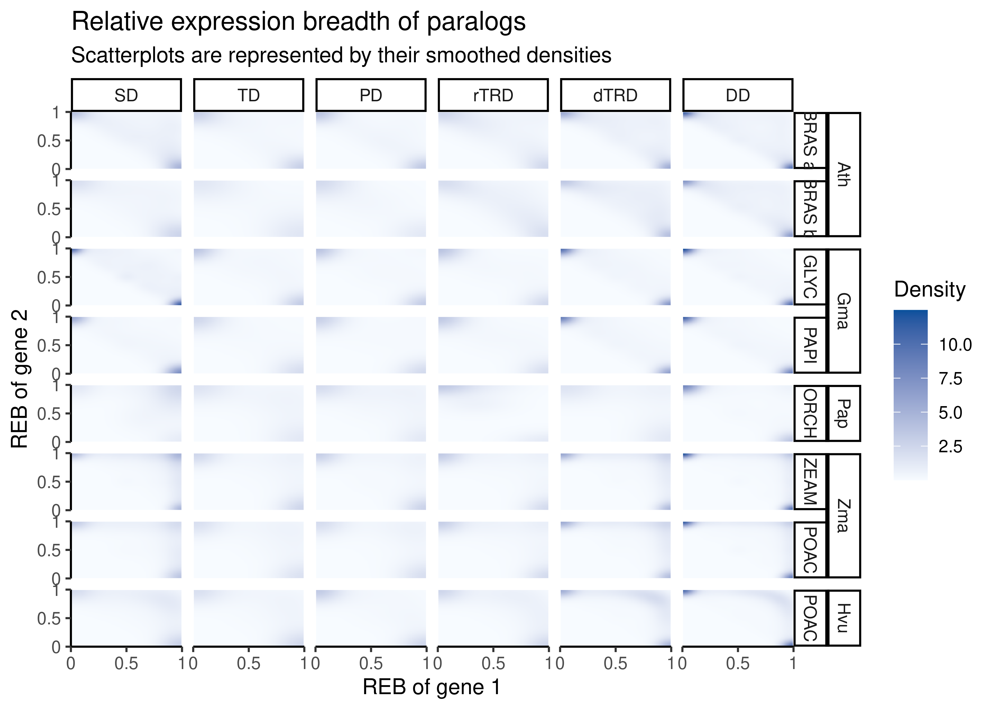

The figure shows that most duplicates diverge asymmetrically. However, for some species (e.g., orchid and maize), a large fraction of segmental duplicates display redundancy at the expression level.

6.2 Comparing relative expression breadth by mode

Next, we will classify gene pairs in three classes based on their relative expression breadths, and then compare the number of genes in each class by duplication mode. The classes and their definitions are:

1. Redundancy: both pairs with REB >0.70.
2. Assymetric divergence: one gene with REB >0.7, and the other gene with REB <0.3.
3. Symmetric divergence: both genes with REB between 0.3 and 0.7.

We will with the classification per se.

# Classify pairs based on REB
reb_classes <- mean_rebs |>
    filter(
        !is.nan(mean_reb1), 
        !is.na(mean_reb1), 
        !is.nan(mean_reb2), 
        !is.na(mean_reb2) 
    ) |>
    mutate(
        class = case_when(
            mean_reb1 >0.7 & mean_reb2 >0.7 ~ "Redundancy",
            mean_reb1 >0.7 & mean_reb2 <0.3 ~ "Asymmetric",
            mean_reb2 >0.7 & mean_reb1 <0.3 ~ "Asymmetric",
            mean_reb1 >0.3 & mean_reb1 <0.7 &
                mean_reb2 > 0.3 & mean_reb2 <0.7 ~ "Symmetric",
            TRUE ~ "Undefined"
        )
    ) |>
    filter(class != "Undefined") |>
    as.data.frame()

Then, we will test for significant associations between each class and duplication modes.

# Test for overrepresentation of REB classes in duplicates from each dup mode
reb_classes_split <- split(reb_classes, reb_classes$species_peak)
ora_dupmode_class <- lapply(reb_classes_split, function(x) {
    
    # Get list of all duplicate pairs
    dups <- x |>
        mutate(pair = str_c(dup1, dup2, sep = "_")) |>
        select(pair, type)
    
    # Get a list of genes for each class
    classes_list <- x |>
        mutate(pair = str_c(dup1, dup2, sep = "_")) |>
        select(pair, class)
    classes_list <- split(classes_list, classes_list$class)
    
    # Perform ORA
    ora_dfs <- lapply(classes_list, function(y) {
        
        df <- HybridExpress::ora(
            genes = unique(y$pair),
            annotation = dups,
            background = dups$pair,
            min_setsize = 2,
            max_setsize = 1e8,
            alpha = 1
        )
        
        return(df)
    }) |>
        bind_rows(.id = "class")
    
    return(ora_dfs)
}) |>
    bind_rows(.id = "species_peak")

Next, we will plot the frequencies of duplicates in each class by mode.

# Plot frequency of duplicates (by mode) in each class
p_reb_classes <- ora_dupmode_class |>
    mutate(
        genes = log10(genes + 1),
        symbol = case_when(
            padj > 0.05 ~ "",
            padj > 0.01 ~ "*",
            padj > 0.001 ~ "**",
            !is.na(padj) ~ "***",
            TRUE ~ NA_character_
        ),
        peak = str_replace_all(species_peak, ".* - peak ", ""),
        species = str_replace_all(species_peak, " - .*", ""),
        species = factor(species, levels = c("Ath", "Gma", "Pap", "Zma", "Hvu")),
        term = factor(term, levels = names(dup_pal)),
        class = factor(class, levels = c("Redundancy", "Symmetric", "Asymmetric"))
    ) |>
    left_join(
        reb_classes |> select(species, peak, peak_name) |>
            distinct() |> mutate(peak = as.character(peak))
    ) |>
    ggplot(aes(x = term, y = class)) +
    geom_tile(aes(fill = genes)) +
    scale_fill_gradient(low = "#E5F5E0", high = "#006D2C") +
    geom_text(aes(label = symbol)) +
    ggh4x::facet_nested(
        cols = vars(species, peak_name)
    ) +
    theme_classic() +
    labs(
        title = "Expression divergence pattern and duplication mode",
        subtitle = "Asterisks indicate significant overrepresentation; P <0.05",
        x = "Duplication mode", y = "Divergence class",
        fill = expression(Log[10] ~ N)
    ) +
    theme(
        legend.position = "bottom",
        axis.text.x = element_text(angle = 90, hjust = 1)
    )

p_reb_classes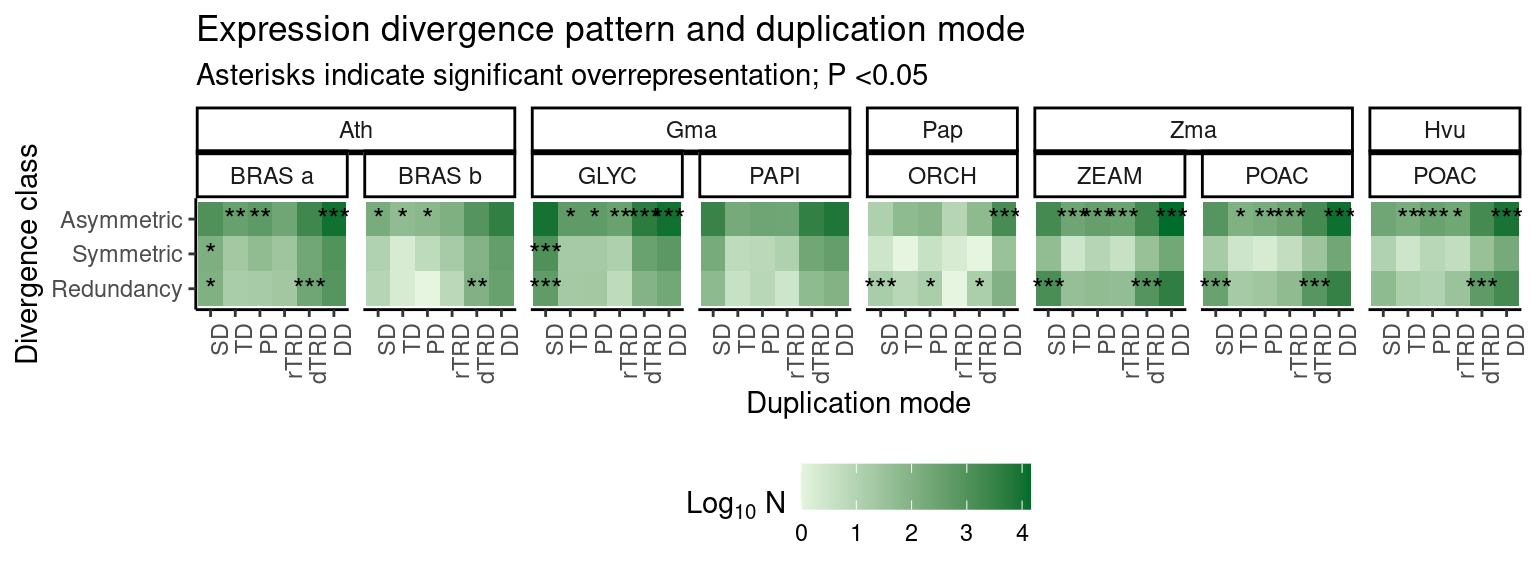

The figure shows that most pairs derived from small-scale duplications (TD, PD, TRD, and DD) are overrepresented in pairs with asymmetric divergence. Segmental duplicates and DNA transposed duplicates are mostly overrepresented in pairs that display redundancy and/or symmetric divergence.

6.3 Do dTRD duplicates display signs of compensatory drift?

Preservation of cis-regulatory landscapes is a quite intuitive mechanism underlying paralog redundancy, and it can explain why segmental duplicates typically become redundant redundancy. However, this is not the only mechanism. Another established hypothesis to explain paralog redundancy relies on the concept of compensatory drift. That is, one copy drifts to lower expression levels, while the other gains higher expression that enables the pair to maintain constant total expression. Here, we will test whether dTRD duplicates (which also display redundancy) show any signs of compensatory drift.

To do that, we will calculate differences in total expression levels for each gene pair across cell types. If differences between dTRD duplicates are greater than differences between other duplicates, this would suggest that dTRD underwent compensatory drift.

# Define helper function to get differences in expression across cell types
exp_diff_cell <- function(spe_list, pairs, cell_type = "cell_type") {
    
    # Get sums across cell types
    exp_sum <- lapply(spe_list, function(spe) {
        return(
            scuttle::aggregateAcrossCells(
                spe, 
                ids = spe[[cell_type]],
                statistics = "sum",
                use.assay.type = "logcounts"
            ) |>
                assay() |>
                as.data.frame() |>
                tibble::rownames_to_column("gene") |>
                pivot_longer(
                    names_to = "cell_type",
                    values_to = "sum_exp",
                    cols = -gene
                ) |>
                as.data.frame()
        )
    }) |>
        bind_rows(.id = "sample") |>
        group_by(gene, cell_type) |> 
        summarise(mean_sums = mean(sum_exp, na.rm = TRUE)) |>
        ungroup() |>
        pivot_wider(
            names_from = cell_type, 
            values_from = mean_sums
        ) |>
        column_to_rownames("gene") |>
        as.matrix()
    
    # For each pair, get difference for each cell type
    diffs <- lapply(seq_len(nrow(pairs)), function(n) {
        
        genes <- c(pairs$dup1[n], pairs$dup2[n])
        fpairs <- NULL
        if(all(genes %in% rownames(exp_sum))) {
            dif_vec <- apply(exp_sum[genes, ], 2, function(x) abs(x[1] - x[2]))
            fpairs <- cbind(pairs[n, ], t(dif_vec))
        }
        
        return(fpairs)
    }) |>
        bind_rows()
    
    return(diffs)
}

# Get differences across cell types
pairs_diffs <- list(
    Ath = exp_diff_cell(spe_all$ath, pairs_age$ath),
    Gma = exp_diff_cell(spe_all$gma, pairs_age$gma, "annotation"),
    Pap = exp_diff_cell(spe_all$pap, pairs_age$pap, "clusters"),
    Zma = exp_diff_cell(spe_all$zma, pairs_age$zma, "cell_type"),
    Hvu = exp_diff_cell(spe_all$hvu, pairs_age$hvu, "tissue")
)

diffs_long <- lapply(pairs_diffs, function(x) {
    x |>
        select(type, peak_name, 6:ncol(x)) |>
        pivot_longer(
            names_to = "cell_type", values_to = "diff", 
            cols = -c(type, peak_name)
        ) |>
        mutate(
            diff = log2(diff + 1),
            type = factor(type, levels = names(dup_pal))
        )
}) |>
    bind_rows(.id = "species") |>
    mutate(
        species_peak = str_c(species, peak_name, sep = "__"),
        species_peak_celltype = str_c(species, peak_name, cell_type, sep = "__")
    )

Next, we will visualize distributions of differences by cell type.

# Get CLDs
clds <- lapply(
    split(diffs_long, diffs_long$species_peak_celltype),
    cld_kw_dunn, value = "diff"
) |>
    bind_rows(.id = "species_peak_celltype") |>
    separate_wider_delim(
        cols = species_peak_celltype, delim = "__", 
        names = c("species", "peak_name", "cell_type")
    ) |>
    mutate(
        species_peak = str_c(species, peak_name, sep = "__"),
        type = factor(Group, levels = names(dup_pal))
    )

# Create one plot for each species and peak
speaks <- unique(clds$species_peak)
p_diffs <- lapply(speaks, function(x) {
    
    p <- diffs_long |>
        filter(species_peak == x) |>
        ggplot(aes(x = diff, y = type)) +
        geom_violin(aes(fill = type)) +
        scale_fill_manual(values = dup_pal) +
        geom_boxplot(width = 0.1, outlier.color = "gray60", outlier.alpha = 0.5) +
        geom_label(
            data = clds |> filter(species_peak == x),
            aes(x = 8, y = Group, label = Letter)
        ) +
        scale_x_continuous(limits = c(0, 10), breaks = c(0, 5, 10)) +
        facet_wrap(vars(cell_type)) +
        theme_classic() +
        theme(
            panel.background = element_rect(fill = bg),
            legend.position = "none"
        ) +
        labs(
            title = "Expression differences between paralogs"
        )
    
    return(p)
})
names(p_diffs) <- speaks

quartose::quarto_tabset(
    content = p_diffs,
    names = gsub("__", " - ", names(p_diffs)), 
    level = 3
)

Ath - BRAS a

Ath - BRAS b

Gma - GLYC

Gma - PAPI

Hvu - POAC

Pap - ORCH

Zma - POAC

Zma - ZEAM

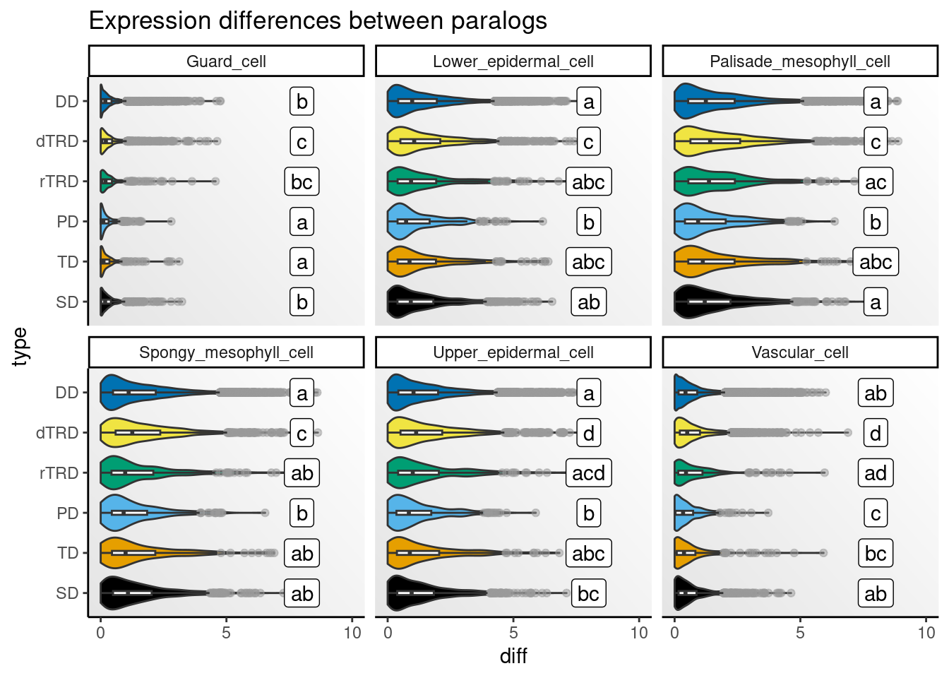
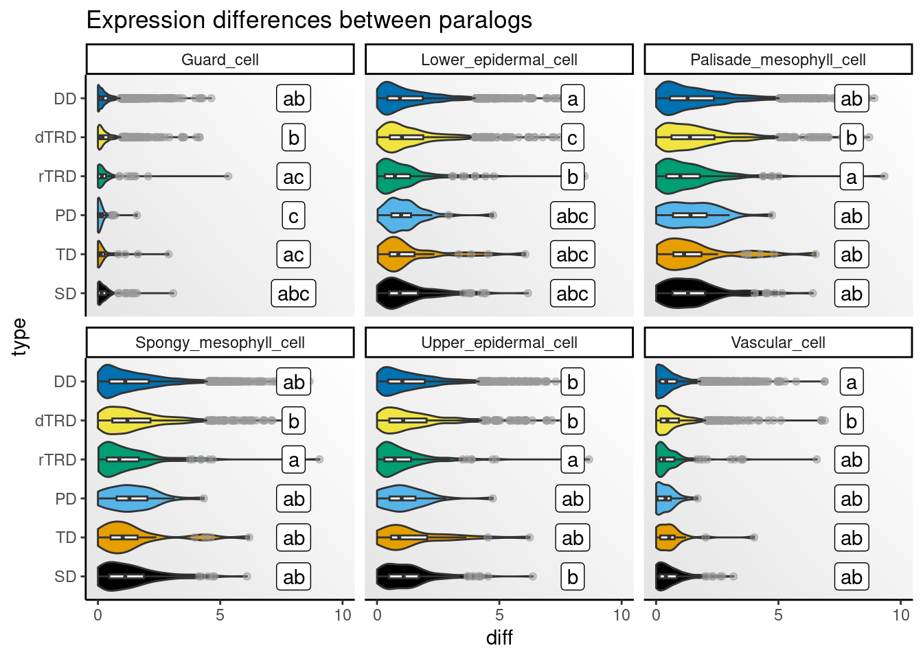
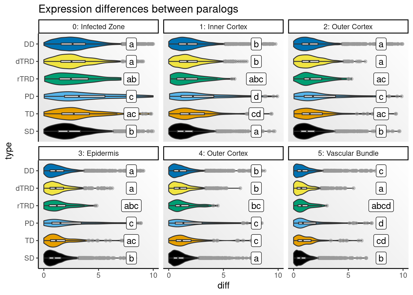
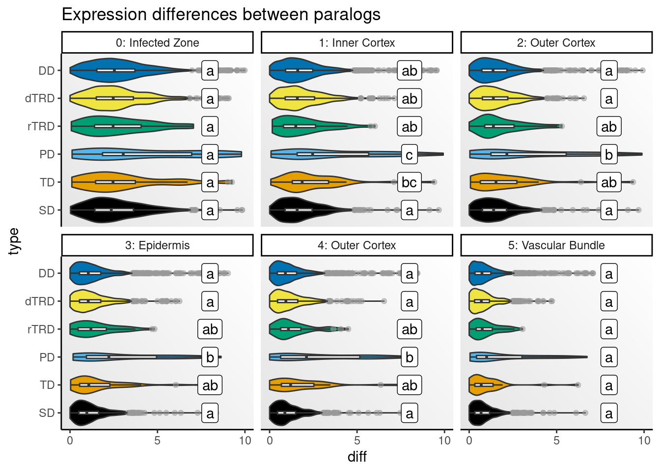
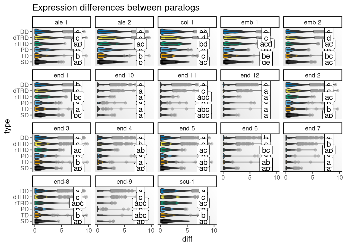
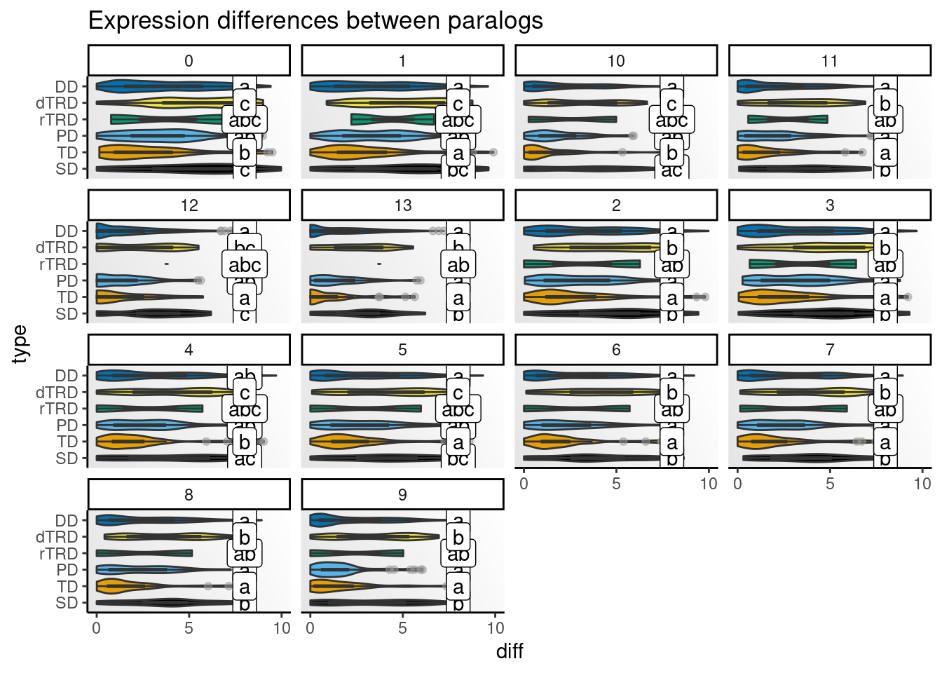
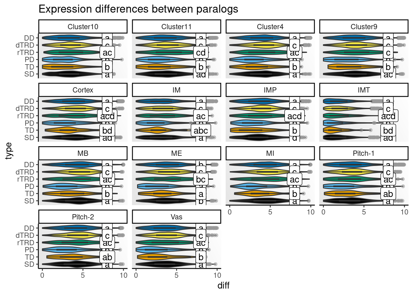
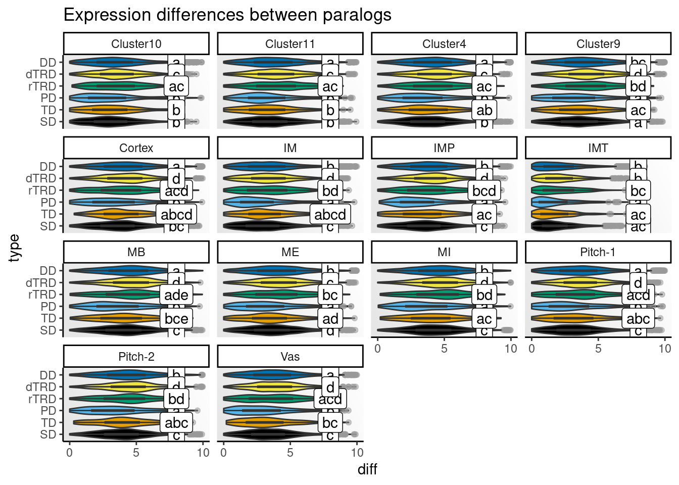
Strikingly, expression differences between paralogs created by DNA tranpositions are consistently larger than differences between paralogs originating from all other duplication modes. This finding provides strong support for compensatory drift as a mechanism driving redundancy among dTRD duplicates.

Saving objects

Finally, we will save important objects to reuse later.

# Objects
## Relative expression breadths
saveRDS(
    rebs, compress = "xz",
    file = here("products", "result_files", "relative_expression_breadth.rds")
)

## Expression differences between paralogs
saveRDS(
    pairs_diffs, compress = "xz",
    file = here("products", "result_files", "paralog_expression_diffs_wide.rds")
)

# Plots
## Smoothed densities of relative expression breadths
saveRDS(
    p_mean_reb, compress = "xz",
    file = here(
        "products", "plots", 
        "smoothed_densities_relative_expression_breadth.rds"
    )
)

## ORA - duplication mode and divergence classes
saveRDS(
    p_reb_classes, compress = "xz",
    file = here("products", "plots", "ORA_dupmode_and_divergence_class.rds")
)

## List of plots with expression differences between paralogs
saveRDS(
    p_diffs, compress = "xz",
    file = here("products", "plots", "expression_differences_paralogs.rds")
)

Session info

This document was created under the following conditions:

─ Session info ───────────────────────────────────────────────────────────────
 setting  value
 version  R version 4.4.1 (2024-06-14)
 os       Ubuntu 22.04.4 LTS
 system   x86_64, linux-gnu
 ui       X11
 language (EN)
 collate  en_US.UTF-8
 ctype    en_US.UTF-8
 tz       Europe/Brussels
 date     2025-08-12
 pandoc   3.2 @ /usr/lib/rstudio/resources/app/bin/quarto/bin/tools/x86_64/ (via rmarkdown)

─ Packages ───────────────────────────────────────────────────────────────────
 package              * version    date (UTC) lib source
 abind                  1.4-5      2016-07-21 [1] CRAN (R 4.4.1)
 backports              1.5.0      2024-05-23 [1] CRAN (R 4.4.1)
 beeswarm               0.4.0      2021-06-01 [1] CRAN (R 4.4.1)
 Biobase              * 2.64.0     2024-04-30 [1] Bioconductor 3.19 (R 4.4.1)
 BiocGenerics         * 0.50.0     2024-04-30 [1] Bioconductor 3.19 (R 4.4.1)
 broom                  1.0.6      2024-05-17 [1] CRAN (R 4.4.1)
 car                    3.1-2      2023-03-30 [1] CRAN (R 4.4.1)
 carData                3.0-5      2022-01-06 [1] CRAN (R 4.4.1)
 cli                    3.6.3      2024-06-21 [1] CRAN (R 4.4.1)
 colorspace             2.1-0      2023-01-23 [1] CRAN (R 4.4.1)
 crayon                 1.5.3      2024-06-20 [1] CRAN (R 4.4.1)
 DelayedArray           0.30.1     2024-05-07 [1] Bioconductor 3.19 (R 4.4.1)
 digest                 0.6.36     2024-06-23 [1] CRAN (R 4.4.1)
 dplyr                * 1.1.4      2023-11-17 [1] CRAN (R 4.4.1)
 evaluate               0.24.0     2024-06-10 [1] CRAN (R 4.4.1)
 farver                 2.1.2      2024-05-13 [1] CRAN (R 4.4.1)
 fastmap                1.2.0      2024-05-15 [1] CRAN (R 4.4.1)
 forcats              * 1.0.0      2023-01-29 [1] CRAN (R 4.4.1)
 generics               0.1.3      2022-07-05 [1] CRAN (R 4.4.1)
 GenomeInfoDb         * 1.40.1     2024-05-24 [1] Bioconductor 3.19 (R 4.4.1)
 GenomeInfoDbData       1.2.12     2024-07-24 [1] Bioconductor
 GenomicRanges        * 1.56.1     2024-06-12 [1] Bioconductor 3.19 (R 4.4.1)
 ggbeeswarm             0.7.2      2023-04-29 [1] CRAN (R 4.4.1)
 ggh4x                  0.2.8      2024-01-23 [1] CRAN (R 4.4.1)
 ggplot2              * 3.5.1      2024-04-23 [1] CRAN (R 4.4.1)
 ggpubr                 0.6.0      2023-02-10 [1] CRAN (R 4.4.1)
 ggsignif               0.6.4.9000 2024-12-12 [1] Github (const-ae/ggsignif@705495f)
 glue                   1.8.0      2024-09-30 [1] https://cran.r-universe.dev (R 4.4.1)
 gtable                 0.3.5      2024-04-22 [1] CRAN (R 4.4.1)
 here                 * 1.0.1      2020-12-13 [1] CRAN (R 4.4.1)
 hms                    1.1.3      2023-03-21 [1] CRAN (R 4.4.1)
 htmltools              0.5.8.1    2024-04-04 [1] CRAN (R 4.4.1)
 htmlwidgets            1.6.4      2023-12-06 [1] CRAN (R 4.4.1)
 httr                   1.4.7      2023-08-15 [1] CRAN (R 4.4.1)
 IRanges              * 2.38.1     2024-07-03 [1] Bioconductor 3.19 (R 4.4.1)
 jsonlite               1.8.8      2023-12-04 [1] CRAN (R 4.4.1)
 knitr                  1.48       2024-07-07 [1] CRAN (R 4.4.1)
 labeling               0.4.3      2023-08-29 [1] CRAN (R 4.4.1)
 lattice                0.22-6     2024-03-20 [1] CRAN (R 4.4.1)
 lifecycle              1.0.4      2023-11-07 [1] CRAN (R 4.4.1)
 lubridate            * 1.9.3      2023-09-27 [1] CRAN (R 4.4.1)
 magick                 2.8.4      2024-07-14 [1] CRAN (R 4.4.1)
 magrittr               2.0.3      2022-03-30 [1] CRAN (R 4.4.1)
 MASS                   7.3-61     2024-06-13 [1] CRAN (R 4.4.1)
 Matrix                 1.7-0      2024-04-26 [1] CRAN (R 4.4.1)
 MatrixGenerics       * 1.16.0     2024-04-30 [1] Bioconductor 3.19 (R 4.4.1)
 matrixStats          * 1.3.0      2024-04-11 [1] CRAN (R 4.4.1)
 munsell                0.5.1      2024-04-01 [1] CRAN (R 4.4.1)
 patchwork              1.3.0      2024-09-16 [1] CRAN (R 4.4.1)
 pillar                 1.10.2     2025-04-05 [1] https://cran.r-universe.dev (R 4.4.1)
 pkgconfig              2.0.3      2019-09-22 [1] CRAN (R 4.4.1)
 purrr                * 1.0.2      2023-08-10 [1] CRAN (R 4.4.1)
 quartose               0.1.0.9000 2025-08-12 [1] Github (djnavarro/quartose@ba8fc0c)
 R6                     2.5.1      2021-08-19 [1] CRAN (R 4.4.1)
 Rcpp                   1.0.13     2024-07-17 [1] CRAN (R 4.4.1)
 readr                * 2.1.5      2024-01-10 [1] CRAN (R 4.4.1)
 rjson                  0.2.21     2022-01-09 [1] CRAN (R 4.4.1)
 rlang                  1.1.4      2024-06-04 [1] CRAN (R 4.4.1)
 rmarkdown              2.27       2024-05-17 [1] CRAN (R 4.4.1)
 rprojroot              2.0.4      2023-11-05 [1] CRAN (R 4.4.1)
 rstatix                0.7.2      2023-02-01 [1] CRAN (R 4.4.1)
 rstudioapi             0.16.0     2024-03-24 [1] CRAN (R 4.4.1)
 S4Arrays               1.4.1      2024-05-20 [1] Bioconductor 3.19 (R 4.4.1)
 S4Vectors            * 0.42.1     2024-07-03 [1] Bioconductor 3.19 (R 4.4.1)
 scales                 1.3.0      2023-11-28 [1] CRAN (R 4.4.1)
 sessioninfo            1.2.2      2021-12-06 [1] CRAN (R 4.4.1)
 SingleCellExperiment * 1.26.0     2024-04-30 [1] Bioconductor 3.19 (R 4.4.1)
 SparseArray            1.4.8      2024-05-24 [1] Bioconductor 3.19 (R 4.4.1)
 SpatialExperiment    * 1.14.0     2024-05-01 [1] Bioconductor 3.19 (R 4.4.1)
 stringi                1.8.4      2024-05-06 [1] CRAN (R 4.4.1)
 stringr              * 1.5.1      2023-11-14 [1] CRAN (R 4.4.1)
 SummarizedExperiment * 1.34.0     2024-05-01 [1] Bioconductor 3.19 (R 4.4.1)
 tibble               * 3.2.1      2023-03-20 [1] CRAN (R 4.4.1)
 tidyr                * 1.3.1      2024-01-24 [1] CRAN (R 4.4.1)
 tidyselect             1.2.1      2024-03-11 [1] CRAN (R 4.4.1)
 tidyverse            * 2.0.0      2023-02-22 [1] CRAN (R 4.4.1)
 timechange             0.3.0      2024-01-18 [1] CRAN (R 4.4.1)
 tzdb                   0.4.0      2023-05-12 [1] CRAN (R 4.4.1)
 UCSC.utils             1.0.0      2024-04-30 [1] Bioconductor 3.19 (R 4.4.1)
 vctrs                  0.6.5      2023-12-01 [1] CRAN (R 4.4.1)
 vipor                  0.4.7      2023-12-18 [1] CRAN (R 4.4.1)
 withr                  3.0.0      2024-01-16 [1] CRAN (R 4.4.1)
 xfun                   0.51       2025-02-19 [1] CRAN (R 4.4.1)
 XVector                0.44.0     2024-04-30 [1] Bioconductor 3.19 (R 4.4.1)
 yaml                   2.3.9      2024-07-05 [1] CRAN (R 4.4.1)
 zlibbioc               1.50.0     2024-04-30 [1] Bioconductor 3.19 (R 4.4.1)

 [1] /home/faalm/R/x86_64-pc-linux-gnu-library/4.4
 [2] /usr/local/lib/R/site-library
 [3] /usr/lib/R/site-library
 [4] /usr/lib/R/library

──────────────────────────────────────────────────────────────────────────────

References

Casneuf, Tineke, Stefanie De Bodt, Jeroen Raes, Steven Maere, and Yves Van de Peer. 2006. “Nonrandom Divergence of Gene Expression Following Gene and Genome Duplications in the Flowering Plant Arabidopsis Thaliana.” Genome Biology 7: 1–11.