# Loading required packages
library(HybridExpress)
library(SummarizedExperiment)
library(tidyverse)
library(here)
library(patchwork)
library(ComplexHeatmap)

set.seed(123) # for reproducibility1 Benchmark 1: allopolyploid and diploid cotton species under salt stress
Here, we will use HybridExpress on data from Dong et al. (2022). In this study, authors compared global transcriptomic responses to modest salinity stress in two allotetraploid cotton species (Gossypium hirsutum and G. mustelinum, AD-genome) relative to their model diploid progenitors (A-genome and D-genome).
1.1 Data description and experimental design
First of all, let’s load the data set we will use here and get to know it. The count matrix and sample metadata are stored in a SummarizedExperiment object in data/se_cotton.rda.
# Load the data
load(here("data", "se_cotton.rda"))

se_cotton
class: SummarizedExperiment
dim: 37505 24
metadata(0):
assays(1): counts
rownames(37505): Gorai.001G000100 Gorai.001G000200 ... Gorai.N028100
Gorai.N028200
rowData names(0):
colnames(24): A2_CK1 A2_CK2 ... AD4_Salt2 AD4_Salt3
colData names(6): species_name species ... sample rep# Taking a look at the assay
head(assay(se_cotton)) A2_CK1 A2_CK2 A2_CK3 A2_Salt1 A2_Salt2 A2_Salt3 D5_CK1 D5_CK2
Gorai.001G000100 150 158 146 72 67 123 0 28
Gorai.001G000200 0 0 0 0 0 0 1 1
Gorai.001G000300 93 101 107 38 47 59 0 24
Gorai.001G000400 9 8 6 7 9 12 2 46
Gorai.001G000500 80 84 99 50 50 71 87 69
Gorai.001G000600 0 0 0 0 0 0 0 0
D5_CK3 D5_Salt1 D5_Salt2 D5_Salt3 AD1_CK1 AD1_CK2 AD1_CK3
Gorai.001G000100 0 1 0 0 10 7 8
Gorai.001G000200 2 5 3 4 10 4 9
Gorai.001G000300 3 2 2 5 16 14 11
Gorai.001G000400 1 2 2 1 19 19 17
Gorai.001G000500 132 201 154 154 100 102 71
Gorai.001G000600 0 0 0 0 0 0 0
AD1_Salt1 AD1_Salt2 AD1_Salt3 AD4_CK1 AD4_CK2 AD4_CK3
Gorai.001G000100 6 3 11 8 11 7
Gorai.001G000200 2 7 5 0 0 1
Gorai.001G000300 7 9 7 9 4 11
Gorai.001G000400 15 33 18 43 47 41
Gorai.001G000500 86 87 104 103 94 93
Gorai.001G000600 0 0 0 0 0 0
AD4_Salt1 AD4_Salt2 AD4_Salt3
Gorai.001G000100 16 7 19
Gorai.001G000200 1 0 1
Gorai.001G000300 7 10 8
Gorai.001G000400 47 42 50
Gorai.001G000500 141 109 112
Gorai.001G000600 0 0 0# Taking a look at the sample metadata
colData(se_cotton) |> as.data.frame() species_name species ploidy condition sample rep
A2_CK1 Garboreum A2 di Control A2_Control 1
A2_CK2 Garboreum A2 di Control A2_Control 2
A2_CK3 Garboreum A2 di Control A2_Control 3
A2_Salt1 Garboreum A2 di Salt A2_Salt 1
A2_Salt2 Garboreum A2 di Salt A2_Salt 2
A2_Salt3 Garboreum A2 di Salt A2_Salt 3
D5_CK1 Graimondii D5 di Control D5_Control 1
D5_CK2 Graimondii D5 di Control D5_Control 2
D5_CK3 Graimondii D5 di Control D5_Control 3
D5_Salt1 Graimondii D5 di Salt D5_Salt 1
D5_Salt2 Graimondii D5 di Salt D5_Salt 2
D5_Salt3 Graimondii D5 di Salt D5_Salt 3
AD1_CK1 Ghirsutum_TM1 AD1 allo Control AD1_Control 1
AD1_CK2 Ghirsutum_TM1 AD1 allo Control AD1_Control 2
AD1_CK3 Ghirsutum_TM1 AD1 allo Control AD1_Control 3
AD1_Salt1 Ghirsutum_TM1 AD1 allo Salt AD1_Salt 1
AD1_Salt2 Ghirsutum_TM1 AD1 allo Salt AD1_Salt 2
AD1_Salt3 Ghirsutum_TM1 AD1 allo Salt AD1_Salt 3
AD4_CK1 Gmustelinum AD4 allo Control AD4_Control 1
AD4_CK2 Gmustelinum AD4 allo Control AD4_Control 2
AD4_CK3 Gmustelinum AD4 allo Control AD4_Control 3
AD4_Salt1 Gmustelinum AD4 allo Salt AD4_Salt 1
AD4_Salt2 Gmustelinum AD4 allo Salt AD4_Salt 2
AD4_Salt3 Gmustelinum AD4 allo Salt AD4_Salt 3Here, we have two hybrid triplets: AD1 (allotetraploid) and its parents A2 and D5 (diploids); and AD4 (allotetraploid) and its parents A2 and D5 (diploids). We also have two conditions: salt stress, and control. Given this experimental design, we will perform comparative transcriptomic analyses for the each triplet separately. For each triplet, we will compare the expression of the allotetraploid with its diploid parents for control and stress conditions separately. In summary, the comparisons will be:
- A2 <-> AD1 <-> D5, control
- A2 <-> AD4 <-> D5, control
- A2 <-> AD1 <-> D5, salt stress
- A2 <-> AD4 <-> D5, salt stress
That said, let’s create subsets of our data set accordingly:
# Get triplets for each allotetraploid species
se_ad1 <- se_cotton[, se_cotton$species %in% c("A2", "D5", "AD1")]
se_ad4 <- se_cotton[, se_cotton$species %in% c("A2", "D5", "AD4")]
1.2 Data processing
Here, we will first remove non-expressed genes (sum of counts <10 across all samples). Then, we will add midparent expression values to each set, and normalize count data by library size.
# Remove non-expressed genes
se_ad1 <- se_ad1[rowSums(assay(se_ad1)) >= 10, ]
se_ad4 <- se_ad4[rowSums(assay(se_ad4)) >= 10, ]

# Add midparent expression
## AD1
se_ad1 <- add_midparent_expression(
    se_ad1,
    coldata_column = "species",
    parent1 = "A2",
    parent2 = "D5"
)

## AD4
se_ad4 <- add_midparent_expression(
    se_ad4,
    coldata_column = "species",
    parent1 = "A2",
    parent2 = "D5"
)

# Normalize data by library size
se_ad1 <- add_size_factors(se_ad1)
se_ad4 <- add_size_factors(se_ad4)
1.3 Exploratory data analyses
Now, we will perform exploratory data analyses to check if samples group together as expected. We will first explore sample clustering with PCA plots.
# Plot PCA
## AD1
se_ad1$species[is.na(se_ad1$species)] <- "midparent"
se_ad1$species[is.na(se_ad1$species)] <- "midparent"

se_ad1$condition[is.na(se_ad1$condition)] <- "-"
se_ad1$condition[is.na(se_ad1$condition)] <- "-"

p_pca1 <- pca_plot(
    se_ad1, color_by = "species", shape_by = "condition", add_mean = TRUE
) + labs(
    title = "PCA of samples - AD1",
    color = "Species",
    shape = "Treatment"
)

## AD4
se_ad4$species[is.na(se_ad4$species)] <- "midparent"
se_ad4$species[is.na(se_ad4$species)] <- "midparent"

se_ad4$condition[is.na(se_ad4$condition)] <- "-"
se_ad4$condition[is.na(se_ad4$condition)] <- "-"

p_pca2 <- pca_plot(
    se_ad4, color_by = "species", shape_by = "condition", add_mean = TRUE
) +
    labs(
        title = "PCA of samples - AD4",
        color = "Species",
        shape = "Treatment"
    )

# Combining plots
p_pca_combined <- patchwork::wrap_plots(
    p_pca1 +
        theme(legend.position = "bottom", legend.box = "vertical"),
    p_pca2 +
        theme(legend.position = "bottom", legend.box = "vertical"),
    nrow = 1
)

p_pca_combined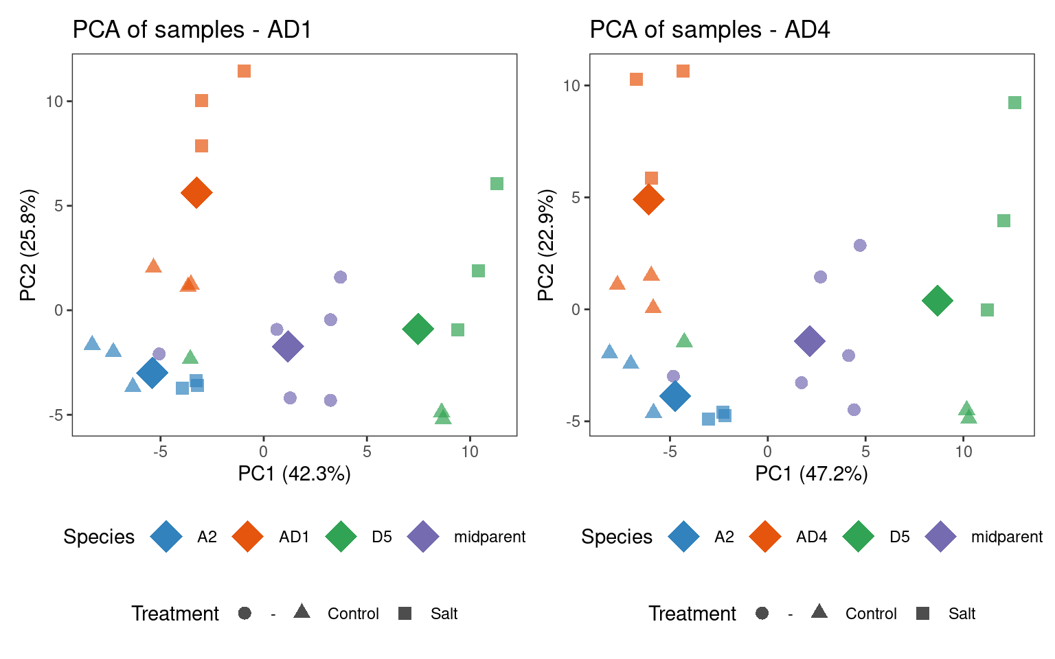
Now, let’s visualize a heatmap of sample correlations.
# Heatmap of sample correlations
## AD1
p_hm1 <- plot_samplecor(
    se_ad1, coldata_cols = c("species", "condition"),
    show_rownames = FALSE
)
p_hm1@column_title <- "AD1"

## AD4
p_hm2 <- plot_samplecor(
    se_ad4, coldata_cols = c("species", "condition"),
    show_rownames = FALSE
)
p_hm2@column_title <- "AD4"

# Combine plots - one per row
patchwork::wrap_plots(
    ggplotify::as.ggplot(p_hm1),
    ggplotify::as.ggplot(p_hm2),
    nrow = 2
)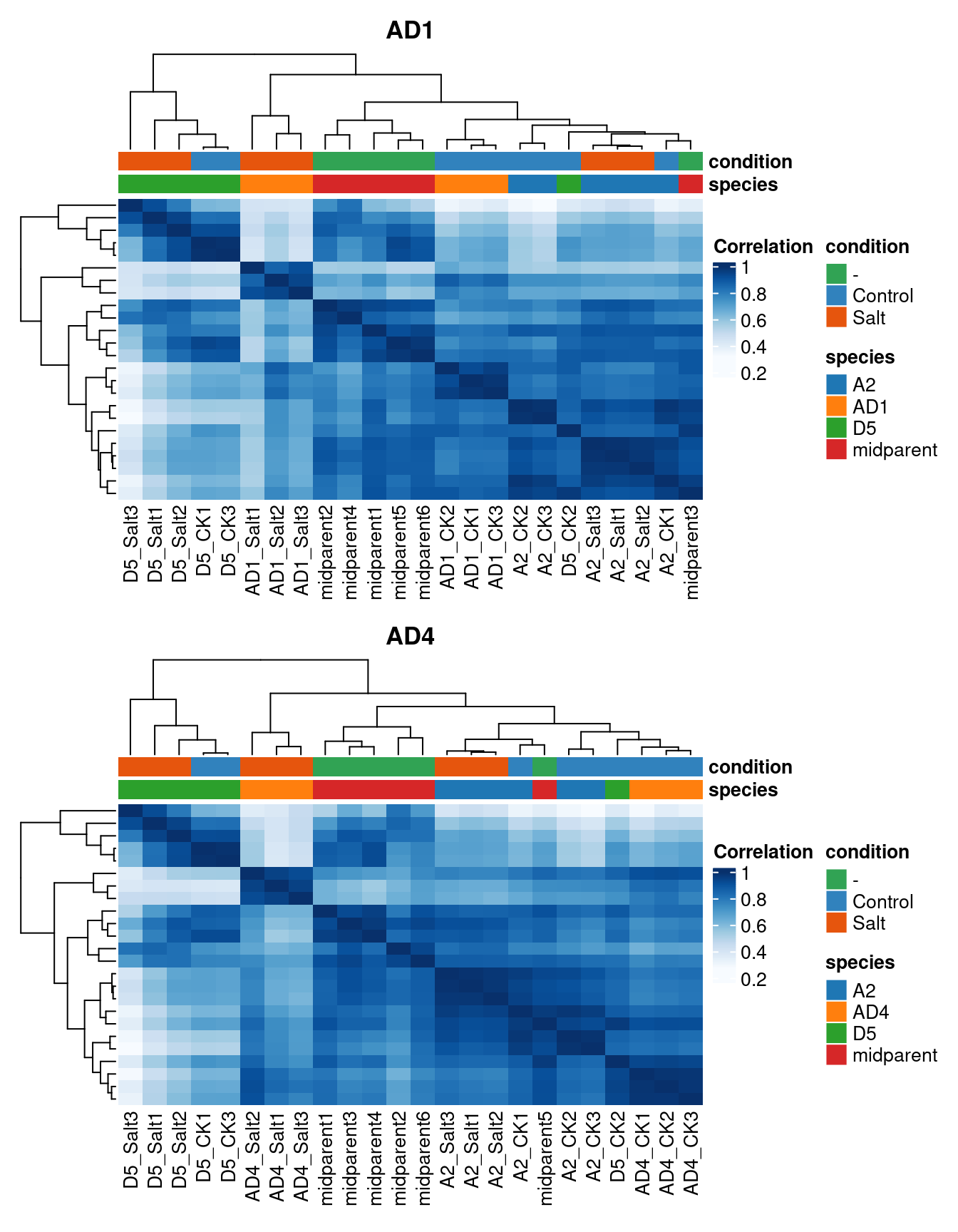
Both plots show that one sample - D5_CK2 - is an outlier. Let’s remove this sample.
# Remove sample D5_CK2 and midparent values
fse_ad1 <- se_ad1[, colnames(se_ad1) != "D5_CK2" & se_ad1$species != "midparent"]
fse_ad4 <- se_ad4[, colnames(se_ad4) != "D5_CK2" & se_ad4$species != "midparent"]
1.4 Identifying differentially expressed genes between species pairs
Here, we will identify differentially expressed genes (DEGs) between pairwise combinations of species in a triplet. For each hybrid, we will do this separately for stress and control samples. We will also recompute midparent values specifically for control and stress samples.
# Get DEGs
## AD1
deg_ad1_control <- add_midparent_expression(
    fse_ad1[, fse_ad1$condition == "Control"],
    coldata_column = "species",
    parent1 = "A2",
    parent2 = "D5"
) |>
    add_size_factors() |>
    get_deg_list(
        coldata_column = "species",
        parent1 = "A2",
        parent2 = "D5",
        offspring = "AD1",
        lfcThreshold = 1
    )

deg_ad1_stress <- add_midparent_expression(
    fse_ad1[, fse_ad1$condition == "Salt"],
    coldata_column = "species",
    parent1 = "A2",
    parent2 = "D5"
) |>
    add_size_factors() |>
    get_deg_list(
        coldata_column = "species",
        parent1 = "A2",
        parent2 = "D5",
        offspring = "AD1",
        lfcThreshold = 1
    )

## AD4
deg_ad4_control <- add_midparent_expression(
    fse_ad4[, fse_ad4$condition == "Control"],
    coldata_column = "species",
    parent1 = "A2",
    parent2 = "D5"
) |>
    add_size_factors() |>
    get_deg_list(
        coldata_column = "species",
        parent1 = "A2",
        parent2 = "D5",
        offspring = "AD4",
        lfcThreshold = 1
    )

deg_ad4_stress <- add_midparent_expression(
    fse_ad4[, fse_ad4$condition == "Salt"],
    coldata_column = "species",
    parent1 = "A2",
    parent2 = "D5"
) |>
    add_size_factors() |>
    get_deg_list(
        coldata_column = "species",
        parent1 = "A2",
        parent2 = "D5",
        offspring = "AD4",
        lfcThreshold = 1
    )
Next, we will visualize the frequencies of DEGs with an expression triangle.
# Plot expression triangle
## AD1
p_triangle_ad1_control <- get_deg_counts(deg_ad1_control) |>
    plot_expression_triangle(
        box_labels = c("A2", "D5", "AD1", "Midparent")
    ) +
    labs(title = "Control") +
    theme(plot.title = element_text(hjust = 0.5))

p_triangle_ad1_stress <- get_deg_counts(deg_ad1_stress) |>
    plot_expression_triangle(
        box_labels = c("A2", "D5", "AD1", "Midparent")
    ) +
    labs(title = "Stress") +
    theme(plot.title = element_text(hjust = 0.5))


## AD4
p_triangle_ad4_control <- get_deg_counts(deg_ad4_control) |>
    plot_expression_triangle(
        box_labels = c("A2", "D5", "AD4", "Midparent"),
        palette = c("dodgerblue3", "firebrick", "darkgoldenrod", "darkgoldenrod3")
    ) +
    labs(title = "Control") +
    theme(plot.title = element_text(hjust = 0.5))


p_triangle_ad4_stress <- get_deg_counts(deg_ad4_stress) |>
    plot_expression_triangle(
        box_labels = c("A2", "D5", "AD4", "Midparent"),
        palette = c("dodgerblue3", "firebrick", "darkgoldenrod", "darkgoldenrod3")
    ) +
    labs(title = "Stress") +
    theme(plot.title = element_text(hjust = 0.5))


# Combine plots
p_triangle_all <- wrap_plots(
    p_triangle_ad1_control,
    p_triangle_ad1_stress,
    p_triangle_ad4_control,
    p_triangle_ad4_stress,
    nrow = 2
) +
    plot_annotation(tag_levels = "A") &
    theme(plot.tag = element_text(size = 16))

p_triangle_all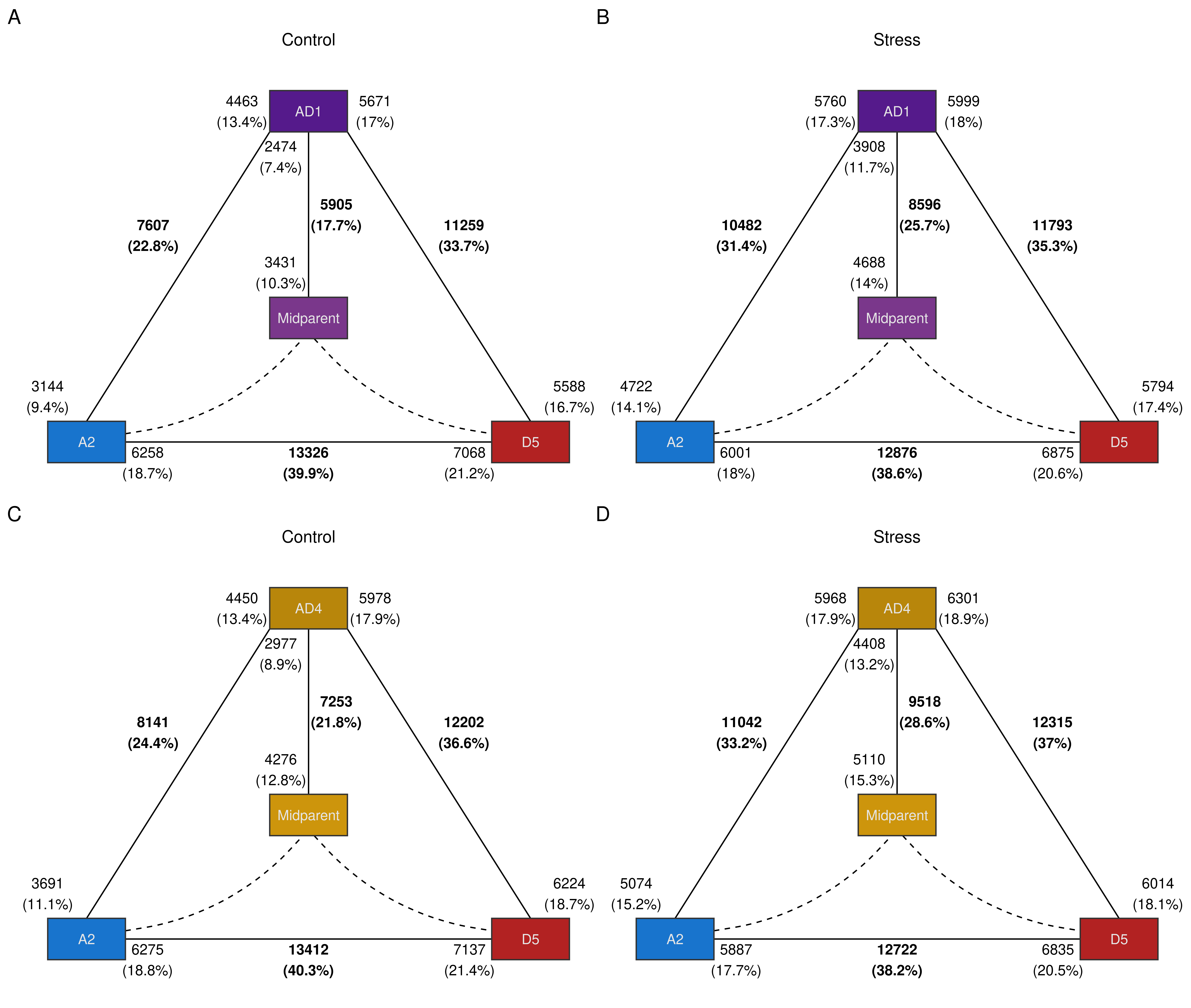
The figure shows two interesting patterns:
In both hybrids and conditions, the number of differentially expressed genes is greater for the hybrids and the D subgenome as compared to the hybrids and the A subgenome. However, such difference is greatly reduced under salt stress.
Overall, salt stress induces an increase in the number of differentially expressed genes relative to both progenitor species.
Next, to better understand the effect of salt stress on subgenome expression bias, we will check if the differentially expressed genes between the hybrids and the parents are the same in control and stress conditions.
# UpSet plot for AD1
ad1 <- list(
    `A, control` = rownames(deg_ad1_control$F1_vs_P1),
    `D, control` = rownames(deg_ad1_control$F1_vs_P2),
    `A, stress` = rownames(deg_ad1_stress$F1_vs_P1),
    `D, stress` = rownames(deg_ad1_stress$F1_vs_P2)
)
m_ad1 <- ComplexHeatmap::make_comb_mat(ad1)

p_upset_ad1 <- ComplexHeatmap::UpSet(
    m_ad1, row_title = "AD1",
    comb_col = ggsci::pal_jama()(7)[comb_degree(m_ad1)],
    top_annotation = upset_top_annotation(m_ad1, add_numbers = TRUE),
    set_order = c("A, control", "A, stress", "D, control", "D, stress")
)

# UpSet plot for AD4
ad4 <- list(
    `A, control` = rownames(deg_ad4_control$F1_vs_P1),
    `D, control` = rownames(deg_ad4_control$F1_vs_P2),
    `A, stress` = rownames(deg_ad4_stress$F1_vs_P1),
    `D, stress` = rownames(deg_ad4_stress$F1_vs_P2)
)
m_ad4 <- ComplexHeatmap::make_comb_mat(ad4)

p_upset_ad4 <- ComplexHeatmap::UpSet(
    m_ad4, row_title = "AD4",
    comb_col = ggsci::pal_jama()(7)[comb_degree(m_ad4)],
    top_annotation = upset_top_annotation(m_ad4, add_numbers = TRUE),
    set_order = c("A, control", "A, stress", "D, control", "D, stress")
)

# Combine UpSet plots into a single, side-by-side plot
p_upset_all <- wrap_plots(
    ggplotify::as.ggplot(p_upset_ad1),
    ggplotify::as.ggplot(p_upset_ad4),
    nrow = 1
) +
    plot_annotation(
        title = "Shared DEGs across conditions and hybrids"
    ) &
    theme(plot.title = element_text(hjust = 0.5))

p_upset_all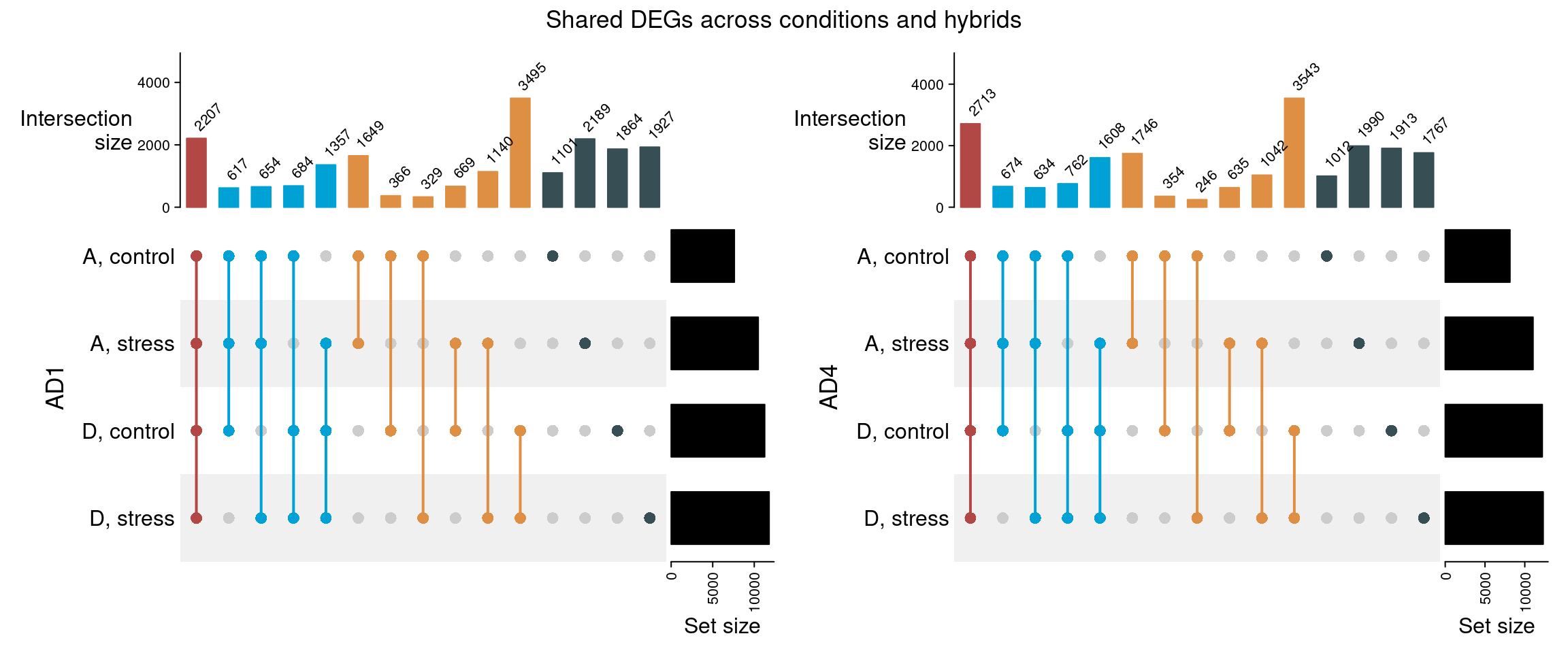
Interestingly, a large number of genes are differentially expressed between the hybrid and the parental genomes for both species (N = 2203 and 2703 for AD1 and AD4, respectively). For DEGs relative to the D subgenome, most of them are shared between control and stress conditions, while for DEGs relative to the A subgenome, most genes are only differentially expressed under salt stress.
1.5 Classifying genes into expression groups
To understand the expression patterns of hybrids relative to their progenitors, we will classify genes onto expression-based categories and classes as in Rapp, Udall, and Wendel (2009).
# Classify genes in expression partitions (classes and categories)
partition_ad1_control <- expression_partitioning(deg_ad1_control)
partition_ad4_control <- expression_partitioning(deg_ad4_control)

partition_ad1_stress <- expression_partitioning(deg_ad1_stress)
partition_ad4_stress <- expression_partitioning(deg_ad4_stress)
Now, let’s visualize results:
# AD1
p_pfreq_ad1_c <- plot_partition_frequencies(
    partition_ad1_control, group_by = "Class", labels = c("A2", "AD1", "D5")
)

p_pfreq_ad1_s <- plot_partition_frequencies(
    partition_ad1_stress, group_by = "Class", labels = c("A2", "AD1", "D5")
)

# AD4
p_pfreq_ad4_c <- plot_partition_frequencies(
    partition_ad4_control, group_by = "Class", labels = c("A2", "AD4", "D5")
)

p_pfreq_ad4_s <- plot_partition_frequencies(
    partition_ad4_stress, group_by = "Class", labels = c("A2", "AD4", "D5")
)

# Combine plots
## Layout: scheme + ((AD1_control + AD1_stress) / (AD4_control + AD4_stress))
p_freq_combined <- wrap_plots(
    p_pfreq_ad1_c[[1]],
    wrap_plots(
        p_pfreq_ad1_c[[2]] + labs(subtitle = "AD1, control", x = NULL),
        p_pfreq_ad1_s[[2]] + labs(subtitle = "AD1, stress", x = NULL),
        p_pfreq_ad4_c[[2]] + labs(subtitle = "AD4, control", x = NULL),
        p_pfreq_ad4_s[[2]] + labs(subtitle = "AD4, stress", x = NULL),
        nrow = 2, ncol = 2
    ),
    ncol = 2,
    widths = c(1, 2)
) &
    theme(plot.margin = unit(c(1, 1, 1, 1), "pt"))

p_freq_combined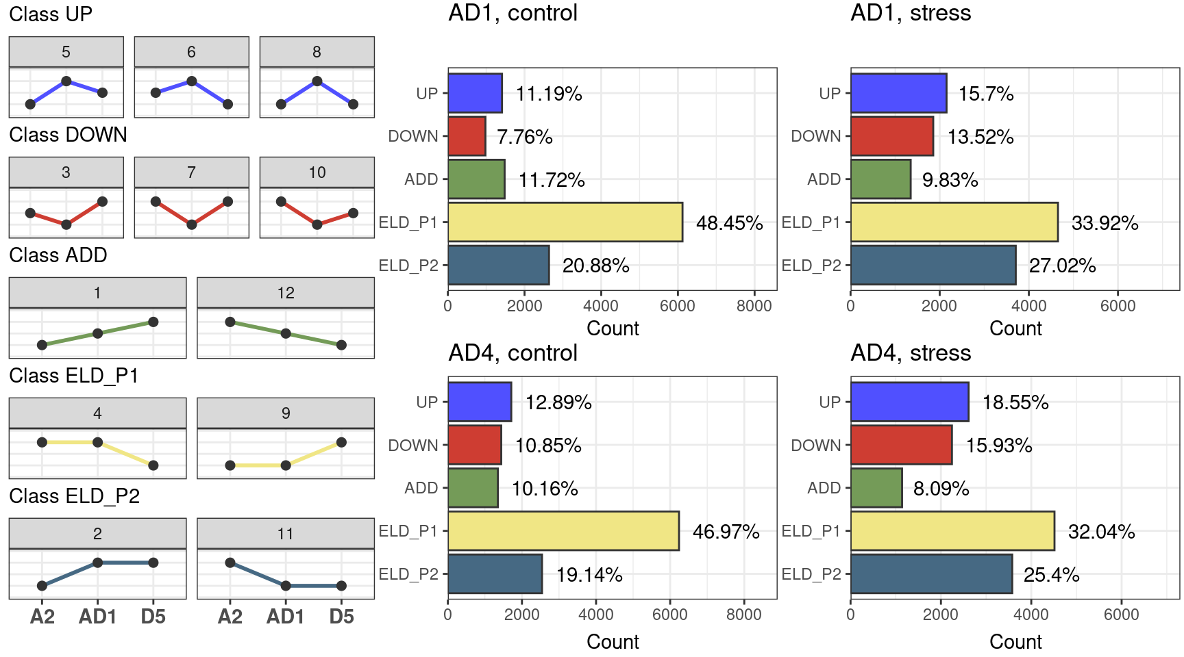
The figure shows that most genes display expression-level dominance towards the parent 1 (A2) in control and stress conditions, both for the AD1 and AD2 allopolyploids. However, for both species, such expression-level dominance is reduced under salt stress.
1.6 Overrepresentation analyses
Now, we will perform overrepresentation analyses of GO terms among genes in each expression class in each condition and species.
# Load GO annotation
load(here("data", "cotton_functions.rda"))
cotton_functions <- lapply(cotton_functions, as.data.frame)

# Perform ORA
## AD1, control
genes_ad1_c <- split(partition_ad1_control$Gene, partition_ad1_control$Class)
ora_ad1_c <- lapply(
    genes_ad1_c, ora,
    annotation = bind_rows(cotton_functions),
    background = rownames(se_ad1),
    min_setsize = 1, max_setsize = 1000
)

## AD1, stress
genes_ad1_s <- split(partition_ad1_stress$Gene, partition_ad1_stress$Class)
ora_ad1_s <- lapply(
    genes_ad1_s, ora,
    annotation = bind_rows(cotton_functions),
    background = rownames(se_ad1),
    min_setsize = 1, max_setsize = 1000
)

## AD4, control
genes_ad4_c <- split(partition_ad4_control$Gene, partition_ad4_control$Class)
ora_ad4_c <- lapply(
    genes_ad4_c, ora,
    annotation = bind_rows(cotton_functions),
    background = rownames(se_ad4),
    min_setsize = 1, max_setsize = 1000
)


## AD4, stress
genes_ad4_s <- split(partition_ad4_stress$Gene, partition_ad4_stress$Class)
ora_ad4_s <- lapply(
    genes_ad4_s, ora,
    annotation = bind_rows(cotton_functions),
    background = rownames(se_ad4),
    min_setsize = 1, max_setsize = 1000
)

# Combining results
cotton_enrichment_all <- bind_rows(
    bind_rows(ora_ad1_c, .id = "Class") |> mutate(group = "AD1_control"),
    bind_rows(ora_ad1_s, .id = "Class") |> mutate(group = "AD1_stress"),
    bind_rows(ora_ad4_c, .id = "Class") |> mutate(group = "AD4_control"),
    bind_rows(ora_ad4_s, .id = "Class") |> mutate(group = "AD4_stress")
) |>
    dplyr::select(class = Class, group, term, genes, all, padj)


# Show results as an interactive table
DT::datatable(
    cotton_enrichment_all,
    selection = "single",
    rownames = FALSE,
    options = list(
        lengthMenu = c(5, 10, 25, 50),
        pageLength = 10
    )
) |>
    DT::formatSignif(columns = "padj", digits = 3)
In summary, this is what we found for each class:
ADD: redox metabolism (cytochrome P450, heme binding, NAD+ nucleosidase activity, oxidoreductase activity, etc). No difference was observed between control and stress conditions.
DOWN: ATP synthesis, aerobic respiration, electron transfer chain, chloroplast thylakoid membrane, organellar ribosome biogenesis, and photosynthesis. Some terms were specific to stress conditions, including cell wall organization, galacturonan metabolism, cellulose synthases, lipid transfer proteins, and glycoside hydrolases family 9.
UP: ribonucleases H domain, cytochrome P450, wall-associated kinases, serine-threonine kinases, peptidases, redox metabolism. Specifically in stress conditions, genes are associated with abscisic acid binding, lectins, glutathione S-transferases, response to salicylic acid, chitinases, leucine-rich repeat (LRR) receptor kinases, pattern recognition receptors, WRKY transcription factors, and systemic acquired resistance.
ELD_P1: in control conditions, genes in this class were associated with chloroplast organization, circadian rhythm, glycine catabolism, photosynthesis, response to wounding, RNA modifications, phosphoglycolate phosphatases, response to water deprivation, ribosome biogenesis, and hydrogen peroxide biosynthesis. In stress conditions, no enrichment was found.
ELD_P2: in control conditions, genes were associated with redox metabolism (heme binding, cytochrome P450, monooxygenase activity, etc). Specifically in stress conditions, genes in this class were associated with alcohol dehydrogenases, coumarin biosynthesis, ERF and WRKY transcription factors, phenylpropanoid biosynthesis, regulation of defense response, and phenylalanine ammonia lyase activity.
Saving important objects
Lastly, we will save important objects to files, so that they can be reused later.
# Plots
save(
    p_freq_combined, compress = "xz",
    file = here("products", "plots", "p_freq_combined.rda")
)

save(
    p_upset_all, compress = "xz",
    file = here("products", "plots", "p_upset_all.rda")
)

save(
    p_pca_combined, compress = "xz",
    file = here("products", "plots", "p_pca_combined.rda")
)

save(
    p_triangle_all, compress = "xz",
    file = here("products", "plots", "p_triangle_all.rda")
)

partition_tables <- list(
    AD1_control = partition_ad1_control,
    AD1_stress = partition_ad1_stress,
    AD4_control = partition_ad4_control,
    AD4_stress = partition_ad4_stress
)

# Objects
partition_tables <- list(
    AD1_control = partition_ad1_control,
    AD1_stress = partition_ad1_stress,
    AD4_control = partition_ad4_control,
    AD4_stress = partition_ad4_stress
)


save(
    partition_tables, compress = "xz",
    file = here("products", "result_files", "partition_tables.rda")
)

save(
    cotton_enrichment_all, compress = "xz",
    file = here("products", "result_files", "cotton_enrichment_all.rda")
)
Session info
This document was created under the following conditions:
─ Session info ───────────────────────────────────────────────────────────────
 setting  value
 version  R version 4.3.2 (2023-10-31)
 os       Ubuntu 22.04.3 LTS
 system   x86_64, linux-gnu
 ui       X11
 language (EN)
 collate  en_US.UTF-8
 ctype    en_US.UTF-8
 tz       Europe/Brussels
 date     2024-03-28
 pandoc   3.1.1 @ /usr/lib/rstudio/resources/app/bin/quarto/bin/tools/ (via rmarkdown)

─ Packages ───────────────────────────────────────────────────────────────────
 package              * version   date (UTC) lib source
 abind                  1.4-5     2016-07-21 [1] CRAN (R 4.3.2)
 Biobase              * 2.62.0    2023-10-24 [1] Bioconductor
 BiocGenerics         * 0.48.1    2023-11-01 [1] Bioconductor
 BiocParallel           1.37.0    2024-01-19 [1] Github (Bioconductor/BiocParallel@79a1b2d)
 bitops                 1.0-7     2021-04-24 [1] CRAN (R 4.3.2)
 bslib                  0.6.1     2023-11-28 [1] CRAN (R 4.3.2)
 cachem                 1.0.8     2023-05-01 [1] CRAN (R 4.3.2)
 Cairo                  1.6-2     2023-11-28 [1] CRAN (R 4.3.2)
 circlize               0.4.15    2022-05-10 [1] CRAN (R 4.3.2)
 cli                    3.6.2     2023-12-11 [1] CRAN (R 4.3.2)
 clue                   0.3-65    2023-09-23 [1] CRAN (R 4.3.2)
 cluster                2.1.5     2023-11-27 [4] CRAN (R 4.3.2)
 codetools              0.2-19    2023-02-01 [4] CRAN (R 4.2.2)
 colorspace             2.1-0     2023-01-23 [1] CRAN (R 4.3.2)
 ComplexHeatmap       * 2.18.0    2023-10-24 [1] Bioconductor
 crayon                 1.5.2     2022-09-29 [1] CRAN (R 4.3.2)
 crosstalk              1.2.1     2023-11-23 [1] CRAN (R 4.3.2)
 DelayedArray           0.28.0    2023-10-24 [1] Bioconductor
 DESeq2                 1.42.0    2023-10-24 [1] Bioconductor
 digest                 0.6.34    2024-01-11 [1] CRAN (R 4.3.2)
 doParallel             1.0.17    2022-02-07 [1] CRAN (R 4.3.2)
 dplyr                * 1.1.4     2023-11-17 [1] CRAN (R 4.3.2)
 DT                     0.31      2023-12-09 [1] CRAN (R 4.3.2)
 ellipsis               0.3.2     2021-04-29 [1] CRAN (R 4.3.2)
 evaluate               0.23      2023-11-01 [1] CRAN (R 4.3.2)
 fansi                  1.0.6     2023-12-08 [1] CRAN (R 4.3.2)
 farver                 2.1.1     2022-07-06 [1] CRAN (R 4.3.2)
 fastmap                1.1.1     2023-02-24 [1] CRAN (R 4.3.2)
 forcats              * 1.0.0     2023-01-29 [1] CRAN (R 4.3.2)
 foreach                1.5.2     2022-02-02 [1] CRAN (R 4.3.2)
 fs                     1.6.3     2023-07-20 [1] CRAN (R 4.3.2)
 generics               0.1.3     2022-07-05 [1] CRAN (R 4.3.2)
 GenomeInfoDb         * 1.38.6    2024-02-08 [1] Bioconductor 3.18 (R 4.3.2)
 GenomeInfoDbData       1.2.11    2023-12-21 [1] Bioconductor
 GenomicRanges        * 1.54.1    2023-10-29 [1] Bioconductor
 GetoptLong             1.0.5     2020-12-15 [1] CRAN (R 4.3.2)
 ggplot2              * 3.5.0     2024-02-23 [1] CRAN (R 4.3.2)
 ggplotify              0.1.2     2023-08-09 [1] CRAN (R 4.3.2)
 ggsci                  3.0.0     2023-03-08 [1] CRAN (R 4.3.2)
 GlobalOptions          0.1.2     2020-06-10 [1] CRAN (R 4.3.2)
 glue                   1.7.0     2024-01-09 [1] CRAN (R 4.3.2)
 gridGraphics           0.5-1     2020-12-13 [1] CRAN (R 4.3.2)
 gtable                 0.3.4     2023-08-21 [1] CRAN (R 4.3.2)
 here                 * 1.0.1     2020-12-13 [1] CRAN (R 4.3.2)
 hms                    1.1.3     2023-03-21 [1] CRAN (R 4.3.2)
 htmltools              0.5.7     2023-11-03 [1] CRAN (R 4.3.2)
 htmlwidgets            1.6.4     2023-12-06 [1] CRAN (R 4.3.2)
 HybridExpress        * 0.99.0    2024-02-15 [1] Bioconductor
 IRanges              * 2.36.0    2023-10-24 [1] Bioconductor
 iterators              1.0.14    2022-02-05 [1] CRAN (R 4.3.2)
 jquerylib              0.1.4     2021-04-26 [1] CRAN (R 4.3.2)
 jsonlite               1.8.8     2023-12-04 [1] CRAN (R 4.3.2)
 knitr                  1.45      2023-10-30 [1] CRAN (R 4.3.2)
 labeling               0.4.3     2023-08-29 [1] CRAN (R 4.3.2)
 lattice                0.22-5    2023-10-24 [4] CRAN (R 4.3.1)
 lifecycle              1.0.4     2023-11-07 [1] CRAN (R 4.3.2)
 locfit                 1.5-9.8   2023-06-11 [1] CRAN (R 4.3.2)
 lubridate            * 1.9.3     2023-09-27 [1] CRAN (R 4.3.2)
 magick                 2.8.2     2023-12-20 [1] CRAN (R 4.3.2)
 magrittr               2.0.3     2022-03-30 [1] CRAN (R 4.3.2)
 Matrix                 1.6-3     2023-11-14 [4] CRAN (R 4.3.2)
 MatrixGenerics       * 1.14.0    2023-10-24 [1] Bioconductor
 matrixStats          * 1.2.0     2023-12-11 [1] CRAN (R 4.3.2)
 memoise                2.0.1     2021-11-26 [1] CRAN (R 4.3.2)
 munsell                0.5.0     2018-06-12 [1] CRAN (R 4.3.2)
 patchwork            * 1.2.0     2024-01-08 [1] CRAN (R 4.3.2)
 pillar                 1.9.0     2023-03-22 [1] CRAN (R 4.3.2)
 pkgconfig              2.0.3     2019-09-22 [1] CRAN (R 4.3.2)
 png                    0.1-8     2022-11-29 [1] CRAN (R 4.3.2)
 purrr                * 1.0.2     2023-08-10 [1] CRAN (R 4.3.2)
 R6                     2.5.1     2021-08-19 [1] CRAN (R 4.3.2)
 RColorBrewer           1.1-3     2022-04-03 [1] CRAN (R 4.3.2)
 Rcpp                   1.0.12    2024-01-09 [1] CRAN (R 4.3.2)
 RCurl                  1.98-1.14 2024-01-09 [1] CRAN (R 4.3.2)
 readr                * 2.1.5     2024-01-10 [1] CRAN (R 4.3.2)
 rjson                  0.2.21    2022-01-09 [1] CRAN (R 4.3.2)
 rlang                  1.1.3     2024-01-10 [1] CRAN (R 4.3.2)
 rmarkdown              2.25      2023-09-18 [1] CRAN (R 4.3.2)
 rprojroot              2.0.4     2023-11-05 [1] CRAN (R 4.3.2)
 rstudioapi             0.15.0    2023-07-07 [1] CRAN (R 4.3.2)
 S4Arrays               1.2.0     2023-10-24 [1] Bioconductor
 S4Vectors            * 0.40.2    2023-11-23 [1] Bioconductor 3.18 (R 4.3.2)
 sass                   0.4.8     2023-12-06 [1] CRAN (R 4.3.2)
 scales                 1.3.0     2023-11-28 [1] CRAN (R 4.3.2)
 sessioninfo            1.2.2     2021-12-06 [1] CRAN (R 4.3.2)
 shape                  1.4.6     2021-05-19 [1] CRAN (R 4.3.2)
 SparseArray            1.2.4     2024-02-11 [1] Bioconductor 3.18 (R 4.3.2)
 stringi                1.8.3     2023-12-11 [1] CRAN (R 4.3.2)
 stringr              * 1.5.1     2023-11-14 [1] CRAN (R 4.3.2)
 SummarizedExperiment * 1.32.0    2023-10-24 [1] Bioconductor
 tibble               * 3.2.1     2023-03-20 [1] CRAN (R 4.3.2)
 tidyr                * 1.3.1     2024-01-24 [1] CRAN (R 4.3.2)
 tidyselect             1.2.0     2022-10-10 [1] CRAN (R 4.3.2)
 tidyverse            * 2.0.0     2023-02-22 [1] CRAN (R 4.3.2)
 timechange             0.3.0     2024-01-18 [1] CRAN (R 4.3.2)
 tzdb                   0.4.0     2023-05-12 [1] CRAN (R 4.3.2)
 utf8                   1.2.4     2023-10-22 [1] CRAN (R 4.3.2)
 vctrs                  0.6.5     2023-12-01 [1] CRAN (R 4.3.2)
 withr                  3.0.0     2024-01-16 [1] CRAN (R 4.3.2)
 xfun                   0.42      2024-02-08 [1] CRAN (R 4.3.2)
 XVector                0.42.0    2023-10-24 [1] Bioconductor
 yaml                   2.3.8     2023-12-11 [1] CRAN (R 4.3.2)
 yulab.utils            0.1.4     2024-01-28 [1] CRAN (R 4.3.2)
 zlibbioc               1.48.0    2023-10-24 [1] Bioconductor

 [1] /home/faalm/R/x86_64-pc-linux-gnu-library/4.3
 [2] /usr/local/lib/R/site-library
 [3] /usr/lib/R/site-library
 [4] /usr/lib/R/library

──────────────────────────────────────────────────────────────────────────────