2  R for evolutionary biology: data structures

R is a very flexible programming language, and it allows developers to create their own data structures (called classes) for their packages. Over the years, some packages have become so popular that the classes they use to store data are now used the “standard” representations for particular types of data. Here, we will show some common data classes in evolutionary biology and comparative genomics research.

2.1 Goals of this lesson

In this lesson, you will learn to:

  • represent and work with sequence data using XString and XStringSet objects
  • represent and work with multiple sequence alignments using XMultipleAlignment objects
  • represent and work with phylogenies using phylo objects

2.2 The Bioconductor ecosystem

The Bioconductor project was created to develop, support, and disseminate free open source software to analyze biological data. It works as a repository of R packages for biological data analysis, with both “core packages” (developed and maintained by the Bioconductor Core Team), and community-contributed packages. We usually refer to Bioconductor as a “package ecosystem” because its packages are tightly integrated and designed for easy interoperation, such that different packages can be used together with minimal effort. An important facilitator of such interoperability is the existence of standardized data structures, such as GRanges objects for genomic coordinates, and DNA/RNA/AAStringSet objects for sequences.

2.2.1 The {Biostrings} package and XStringSet objects

The Biostrings package (Pagès et al. 2022) allows efficient manipulation of biological sequences, and its data classes are standard for all Bioconductor packages that involve sequence analyses. The data classes in Biostrings to represent sets of biological sequences are:

  1. DNAStringSet: for sets of DNA strings.
  2. RNAStringSet: for sets of RNA strings.
  3. AAStringSet: for sets of amino acid strings.

For a single sequence, the each of the above has a correspoding XString class (i.e., DNAString, RNAString, AAString). For example, let’s create some XString objects manually:

library(Biostrings)

# Create `DNAString` object
dna_seq <- DNAString("ATGGCCGACTCA")
dna_seq
12-letter DNAString object
seq: ATGGCCGACTCA
# Convert `DNAString` to `RNAString`
rna_seq <- RNAString(dna_seq)
rna_seq
12-letter RNAString object
seq: AUGGCCGACUCA
# Translate `RNAString` to create `AAString`
aa_seq <- translate(rna_seq)
aa_seq
4-letter AAString object
seq: MADS

In real-world data analyses, we would work with multiple sequences (e.g., a whole genome or a whole proteome). Multiple sequences are stored in XStringSet objects, which can be read from FASTA files with readXStringSet() functions, namely:

  1. readDNAStringSet(): read FASTA file containing multiple DNA sequences.
  2. readRNAStringSet(): read FASTA file containing multiple RNA sequences.
  3. readAAStringSet(): read FASTA file containing multiple AA sequences.

For example, let’s read an example FASTA file that come with the Biostrings package.

# Path to FASTA file containing an ORF
fasta_file <- system.file("extdata", "someORF.fa", package = "Biostrings")
fasta_file
[1] "/home/runner/work/_temp/Library/Biostrings/extdata/someORF.fa"
# Read FASTA file as a DNAStringSet object
dna_seqs <- readDNAStringSet(fasta_file)
dna_seqs
DNAStringSet object of length 7:
    width seq                                               names               
[1]  5573 ACTTGTAAATATATCTTTTATTT...CTTATCGACCTTATTGTTGATAT YAL001C TFC3 SGDI...
[2]  5825 TTCCAAGGCCGATGAATTCGACT...AGTAAATTTTTTTCTATTCTCTT YAL002W VPS8 SGDI...
[3]  2987 CTTCATGTCAGCCTGCACTTCTG...TGGTACTCATGTAGCTGCCTCAT YAL003W EFB1 SGDI...
[4]  3929 CACTCATATCGGGGGTCTTACTT...TGTCCCGAAACACGAAAAAGTAC YAL005C SSA1 SGDI...
[5]  2648 AGAGAAAGAGTTTCACTTCTTGA...ATATAATTTATGTGTGAACATAG YAL007C ERP2 SGDI...
[6]  2597 GTGTCCGGGCCTCGCAGGCGTTC...AAGTTTTGGCAGAATGTACTTTT YAL008W FUN14 SGD...
[7]  2780 CAAGATAATGTCAAAGTTAGTGG...GCTAAGGAAGAAAAAAAAATCAC YAL009W SPO7 SGDI...

Some examples of what you can do to explore XStringSet objects include:

# width(): get sequence lengths
width(dna_seqs)
[1] 5573 5825 2987 3929 2648 2597 2780
# names(): get sequence names
names(dna_seqs)
[1] "YAL001C TFC3 SGDID:S0000001, Chr I from 152168-146596, reverse complement, Verified ORF"
[2] "YAL002W VPS8 SGDID:S0000002, Chr I from 142709-148533, Verified ORF"                    
[3] "YAL003W EFB1 SGDID:S0000003, Chr I from 141176-144162, Verified ORF"                    
[4] "YAL005C SSA1 SGDID:S0000004, Chr I from 142433-138505, reverse complement, Verified ORF"
[5] "YAL007C ERP2 SGDID:S0000005, Chr I from 139347-136700, reverse complement, Verified ORF"
[6] "YAL008W FUN14 SGDID:S0000006, Chr I from 135916-138512, Verified ORF"                   
[7] "YAL009W SPO7 SGDID:S0000007, Chr I from 134856-137635, Verified ORF"                    
# subset DNAStringSet and create a DNAStringSet of length 1
dna_seqs[1]
DNAStringSet object of length 1:
    width seq                                               names               
[1]  5573 ACTTGTAAATATATCTTTTATTT...CTTATCGACCTTATTGTTGATAT YAL001C TFC3 SGDI...
# subset DNAStringSet and create a DNAString object
dna_seqs[[1]]
5573-letter DNAString object
seq: ACTTGTAAATATATCTTTTATTTTCCGAGAGGAAAA...AATTTCTTAAACGCTTATCGACCTTATTGTTGATAT

All functions above would also work for AAStringSet objects and RNAStringSet objects.

Exercises

Use the dna_seqs object created above to answer the following questions:

  1. What is the length of the 3rd sequence?
  2. What is the name of the 5th sequence?
  3. How many times does the TTCC sequence string occur in each sequence? Hint: use the function vcountPattern().
  4. What are the first 3 nucleotides of each sequence? Hint: use the subseq() function.
# Q1: Length of the 3rd sequence
width(dna_seqs)[3]
[1] 2987
# Q2: Name of the 5th sequence
names(dna_seqs)[5]
[1] "YAL007C ERP2 SGDID:S0000005, Chr I from 139347-136700, reverse complement, Verified ORF"
# Q3: Minimum and maximum temperature
vcountPattern("TTCC", dna_seqs)
[1] 21 28 16 23 15  8  5
# Q4: First 3 nucleotides of each sequence
subseq(dna_seqs, start = 1, end = 3)
DNAStringSet object of length 7:
    width seq                                               names               
[1]     3 ACT                                               YAL001C TFC3 SGDI...
[2]     3 TTC                                               YAL002W VPS8 SGDI...
[3]     3 CTT                                               YAL003W EFB1 SGDI...
[4]     3 CAC                                               YAL005C SSA1 SGDI...
[5]     3 AGA                                               YAL007C ERP2 SGDI...
[6]     3 GTG                                               YAL008W FUN14 SGD...
[7]     3 CAA                                               YAL009W SPO7 SGDI...

2.2.2 The {Biostrings} package and XMultipleAlignment objects

Like XStringSet objects, XMultipleAlignment objects also store sequences, but sequences that were aligned using a Sequence Alignment algorithm. FASTA files containing aligned sequences can be read with XMultipleAlignment functions, namely:

  1. readDNAMultipleAlignment(): read a FASTA file containing aligned DNA sequences.
  2. readRNAMultipleAlignment(): read a FASTA file containing aligned RNA sequences.
  3. readAAMultipleAlignment(): read a FASTA file containing aligned amino acid sequences.

For example:

# Path to FASTA file containing MSA of DNA sequences
aln_path <- system.file("extdata", "msx2_mRNA.aln", package = "Biostrings")
aln_path
[1] "/home/runner/work/_temp/Library/Biostrings/extdata/msx2_mRNA.aln"
# Read MSA file
dna_msa <- readDNAMultipleAlignment(aln_path)
dna_msa
DNAMultipleAlignment with 8 rows and 2343 columns
     aln                                                    names               
[1] -----TCCCGTCTCCGCAGCAAAAAA...TCACAATTAAAAAAAAAAAAAAAAA gi|84452153|ref|N...
[2] --------------------------...------------------------- gi|208431713|ref|...
[3] --------------------------...------------------------- gi|118601823|ref|...
[4] ----------------------AAAA...------------------------- gi|114326503|ref|...
[5] --------------------------...------------------------- gi|119220589|ref|...
[6] --------------------------...------------------------- gi|148540149|ref|...
[7] --------------CGGCTCCGCAGC...------------------------- gi|45383056|ref|N...
[8] GGGGGAGACTTCAGAAGTTGTTGTCC...------------------------- gi|213515133|ref|...
Exercises

What is the consensus sequence of the multiple sequence alignment in dna_msa? Hint: use the consensusString() function.

consensusString(dna_msa)
[1] "----------------------VWVMKYYBSRSTSDYVVMDKBHSVGHKSMSVRYVKDRYHRHKVSBYDNVVRVYWMSYNGVRCRGABAMGTCA-YRGCTTCTCYGTSCAWAGGCRRTGRCYTGTTYTCGYCCRRYGARGAGGGCCCVGCRGTKSTSGCCSGMCSRGGCCCVGGGCCYGGRGGMGCCGAGGGVGSCGMRGAGGAGCRCMRSGTCAAGGTCTCCAGCYTGCCCTTCAGYGTGGAGGCGCTCATGTCSGACAAGAARCCGCCYAAGGARKCGYCSSCGSKGCCRSCCGAMWGCGSCTCSGCYGGSGCYRYCCTGSGG----CCR-----CTGCTGCTGYCGGGVCACGGCGYYCGG-GAMGCKCMCAGYCCC---GGGCCKCTSGTSAARMCCTTCGAGACCGCCTCGGTCAAGTCGGARAAYTCMGARGAYGGARCGBCGTGGATVCAGGARCCCGGCMGATAYTCSCCKCCGCCMAGACAYATGAGCCCYACMRCCTGCACCCTGMGGAARCACAAGACCAAYCGGAAGCCVCGCACVCCCTTYACCACRTCCCAGCTYCTVGCCYTGGAGCGCAAGTTCCGYCAGAAACAGTACCTSTCCATYGCAGAGCGKGCMGAGTTCTCCAGCTCYCTGAACCTYACAGAGACCCAGGTCAAAATCTGGTTCCARAAYCGAAGGGCYAAGGCSAARAGACTGCAGGAGGCRGARCTRGARAAGCTSAARATGGCTGCMAARCCTATGYTGCCCTCVRGCTTCAGYCTBCCYTTCCCYATCARCTCSCCCYTGCARGCRGCRTCCMTATAYGGMRCRTCYTACCCBTTYCATAGACCTGTGC---TYCCYATCCCGCCYGT-BGGACTCTATGCSACBCCRGTSGGATATRGCATGTACCAYCTRTCCTAAGGAAGACCAGATSRRY-MGACTCCAGGATGGRTGWYTGYYTRAWAGMMTYYCCCNTCCMKCTYCRAGAAKGCRGTRCCAAYYY-TRSWMCTGMA-YGCWARCYYTGCRT-YGTCACCCTAASCRDCWRGGCTG--RCAGGRCYACWYGAYAYAGADBVAATTTGTTMTKTAGGYRRSAGRCACY-AAGMCYKGKTTTSTTKKYATARTYYYCYRRRTGC--CCCCTTTTCCYYTCASARW-KATTGGCTCTGMTAGTTTTTATGTATAAATATATA------ATAAAATATAAKAC--TTTTTATAYRSCARATGTAAAAATTCAAVYTRTKYTRDAW--GSCAAARTTTRTWKRHWYRYKTVBYHDKWTW---------YVTRKVTMDSMTYHYYHHMWRAHWHYSWGW-WAGYYC---------------------------------------------------------------------------------------------------------------------------------------------------------------------------------------------------------------------------------------------------------------------------------------------------------------------------------------------------------------------------------------------------------------------------------------------------------------------------------------------------------------------------------------------------------------------------------------------------------------------------------------------------------------------------------------------------------------------------------------------------------------------------------------------------------------------------------------------------------------------------------------------------------------------------------------------------------------------------------------------------------------------------------------------------"

2.3 The {ape} package and phylo objects

The ape package (Paradis and Schliep 2019) is one of the most popular packages for Analyses of Phylogenetics and Evolution (from where the name comes), and it represents phylogenies as phylo objects. Because of ape’s popularity, phylo objects have become the standard data structure for phylogenies in R.

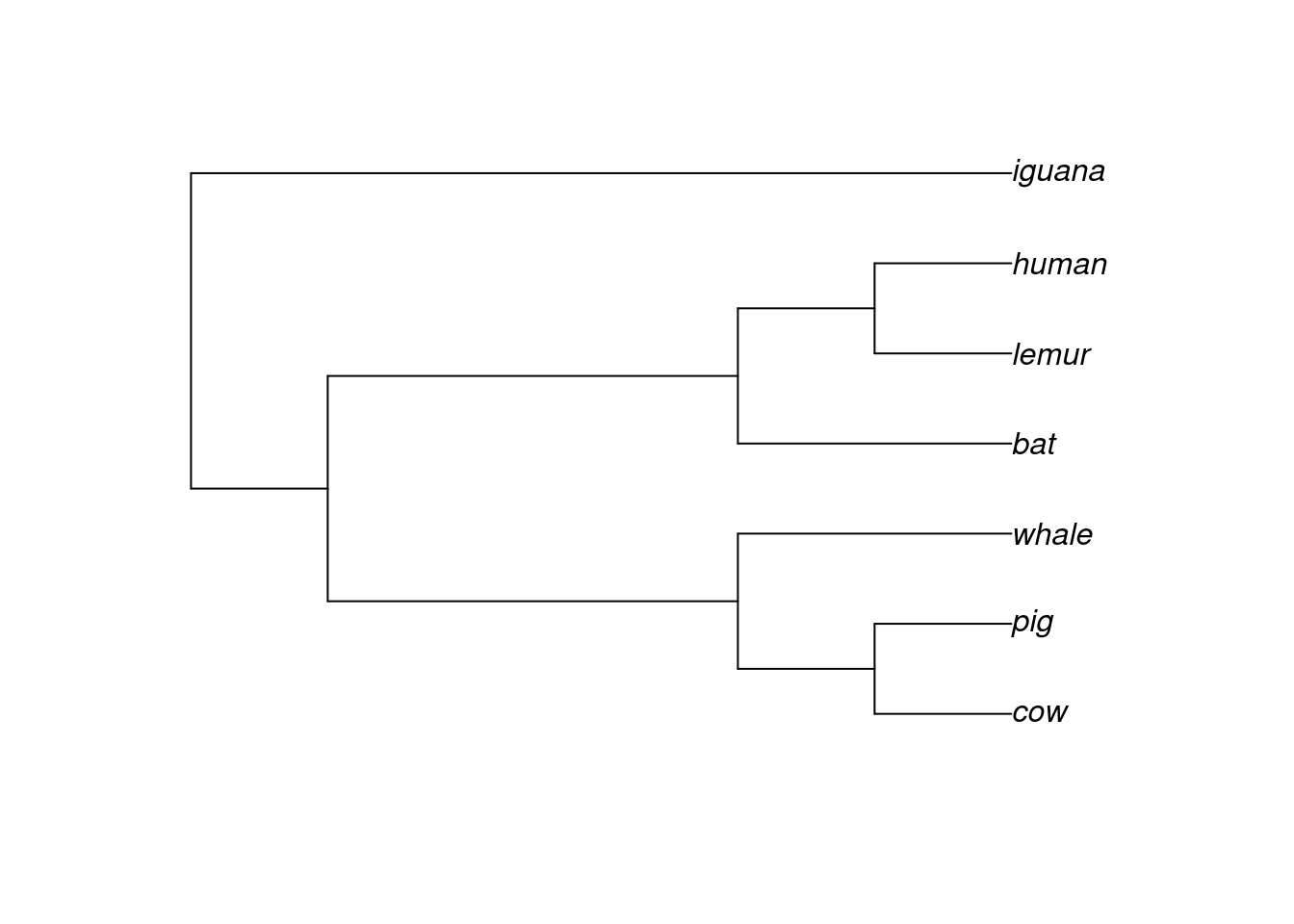
To create phylo objects, you will use the function read.tree(), which accepts both the path to a file containing the tree (in Newick format, for example), or a text representation of a phylogeny. To demonstrate the structure of a phylo object, let’s create a phylogeny from text:

library(ape)

# Create tree from text
text_tree <- "((((cow, pig),whale), (bat, (lemur, human))), iguana);"
tree <- read.tree(text = text_tree)

tree

Phylogenetic tree with 7 tips and 6 internal nodes.

Tip labels:
  cow, pig, whale, bat, lemur, human, ...

Rooted; no branch lengths.

This is what a phylo object looks like. In a sense, a phylo object is a list, a standard R data structure, but with some standard elements. Let’s explore them:

# Structure of the `phylo` object
str(tree)
List of 3
 $ edge     : int [1:12, 1:2] 8 9 10 11 11 10 9 12 12 13 ...
 $ Nnode    : int 6
 $ tip.label: chr [1:7] "cow" "pig" "whale" "bat" ...
 - attr(*, "class")= chr "phylo"
 - attr(*, "order")= chr "cladewise"
# Exploring each element individually
tree$edge
      [,1] [,2]
 [1,]    8    9
 [2,]    9   10
 [3,]   10   11
 [4,]   11    1
 [5,]   11    2
 [6,]   10    3
 [7,]    9   12
 [8,]   12    4
 [9,]   12   13
[10,]   13    5
[11,]   13    6
[12,]    8    7
tree$Nnode
[1] 6
tree$tip.label
[1] "cow"    "pig"    "whale"  "bat"    "lemur"  "human"  "iguana"

As phylo objects have become standard, there are hundreds of functions (from dozens of packages) that were especially designed to work on phylo objects. For example, if you want to plot the tree, you would use the plot() function:

# Plot tree
plot(tree)

We will explore other examples in future lessons.

Exercises

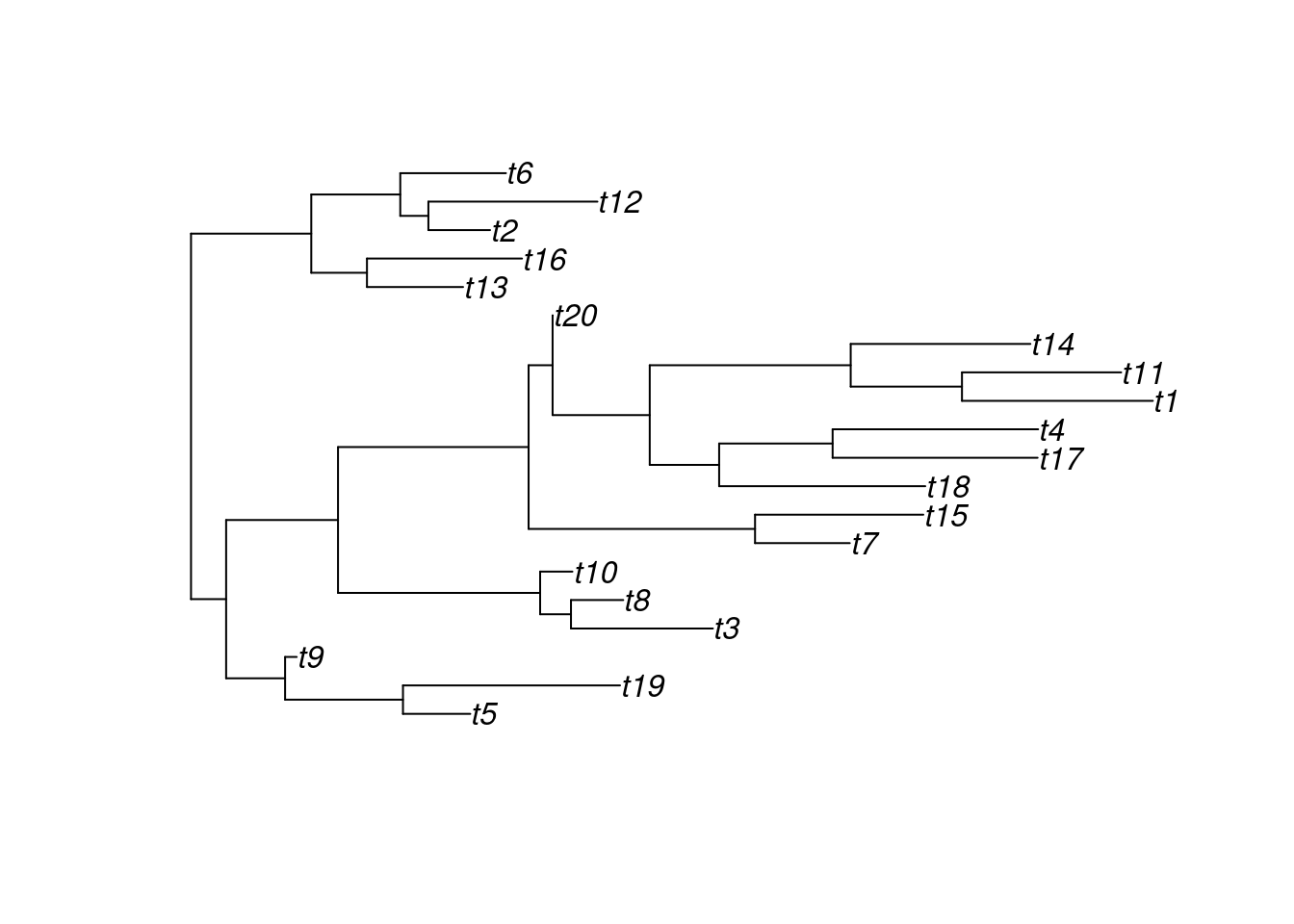
Use the following code to simulate a random tree and answer the questions below:

set.seed(123) # for reproducibility
sim_tree <- rtree(n = 20)
  1. How many terminal taxa (i.e., tips) are there?
  2. What the the names of terminal taxa?
  3. What taxon is more closely-related to the taxon “t1”?
# Q1: Number of terminal taxa
Ntip(sim_tree)
[1] 20
# Q2: Names of terminal taxa
sim_tree$tip.label
 [1] "t5"  "t19" "t9"  "t3"  "t8"  "t10" "t7"  "t15" "t18" "t17" "t4"  "t1" 
[13] "t11" "t14" "t20" "t13" "t16" "t2"  "t12" "t6" 
# Q3: Visualizing the tree to check who is more closely-related to 't1'
plot(sim_tree)

References

Pagès, H., P. Aboyoun, R. Gentleman, and S. DebRoy. 2022. Biostrings: Efficient Manipulation of Biological Strings. https://bioconductor.org/packages/Biostrings.
Paradis, Emmanuel, and Klaus Schliep. 2019. “Ape 5.0: An Environment for Modern Phylogenetics and Evolutionary Analyses in R.” Bioinformatics 35: 526–28. https://doi.org/10.1093/bioinformatics/bty633.